Post Alignment Visualization
View some of our alignments in IGV
Let’s take a look at some of the aligments we just produced using IGV. Since we have configured our AWS instances to serve all of the files produced by the exercises we can load our BAM files by URL. Since the BAM files are indexed, only the information we request to view will be transferred from the AWS instance to our browser for viewing.
To load the exome BAMs your URLs should look like these (don’t forget to substitute your number for #):
- http://s#.pmbio.org/align/Exome_Norm_sorted_mrkdup_bqsr.bam
- http://s#.pmbio.org/align/Exome_Tumor_sorted_mrkdup_bqsr.bam
Let’s go through some simple exercises for exploring the Exome BAMs in IGV.
Load the exome BAMs
- If IGV is already running, start a new session with
File->New Session - Load the bam files (using the URLs above) with
File->Load from URL - Rename the tracks (e.g., Exome Norm Coverage, Exome Norm BAM, Exome Tumor Coverage, Exome Tumor BAM) by right-clicking on each track and selecting
Rename Track - Save session with
File->Save Session
View exome alignments for an example gene
For example, let’s take a look at TP53 on chr17. Simply type TP53 into the search box and hit Go or enter.
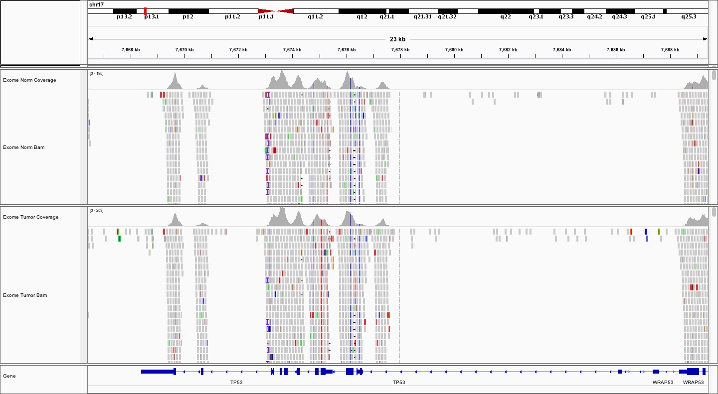
Notice the coverage peaks roughly centered around each protein-coding exon. Notice that there are several variants.
EXERCISE
Explore the TP53 sequence and answer the following questions. How many potential variants can you find? Are they SNVs or indels? Are they coding or non-coding? Are the homozygous or heterozygous? Are they germline or somatic? How can you tell?
Hint
Expand the Gene track to see where TP53 starts. In the collapsed view it appears to be contiguous with WRAP53 due to overlapping transcripts.
Hint
Zoom into the ~7-8kb region with coding exons (thicker than UTR). Look for colored bars in the coverage track for SNVs and stacks of black gaps (deletions) or purple bars (insertions).
Answer
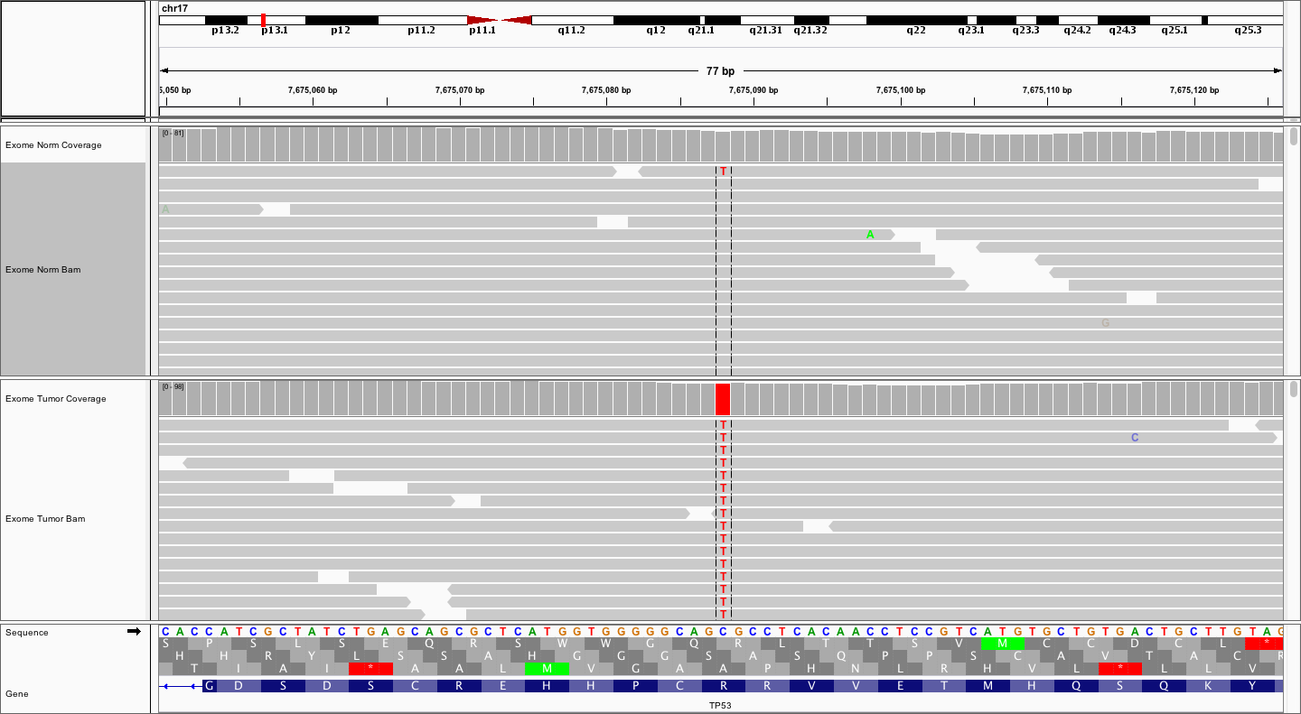
There appear to be at least 5 SNVs, 1 insertion and 3 deletions. Two of the SNVs are in coding exons while the rest of the variants are intronic. Note: The 4 indels all look like potential artifacts due to their proximity to homopolymer stretches or repetitive sequences. All of the SNVs appear real and homozygous (or hemizygous). One SNV appears to be somatic. In all cases the VAFs of the SNVs are at or near 100% and one of them is only observed in the tumor.
This is one the variants you should have found in TP53. Which one?
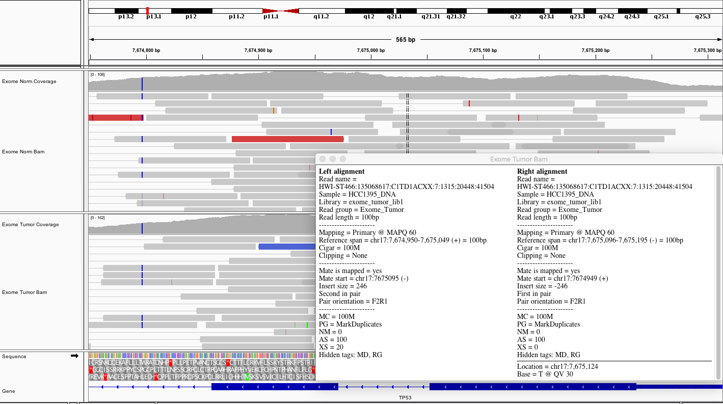
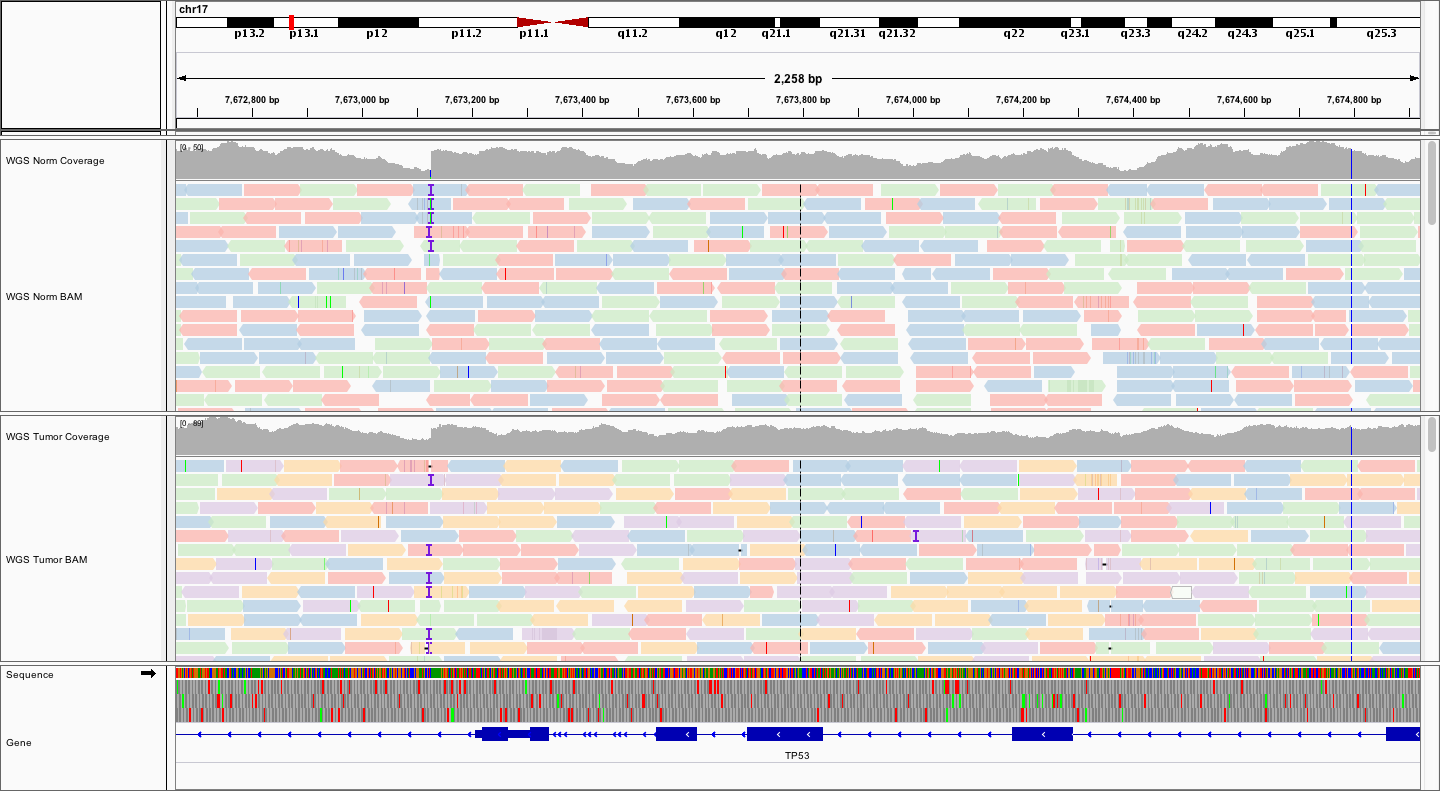
Now, try viewing the reads as read pairs. How big do your fragments look?
Answer
The fragment sizes vary. But, estimating by eye, and clicking on a few read pairs to get the insert size, it appears that fragments are in the 200-500bp range
Here is a representative region showing reads in paired mode.
Considering TP53, what does the average coverage look like?
Hint
The exons of TP53 have coverage peaks ranging from ~100 to 200X. On average there appears to be ~150X coverage for coding exons.
Try loading the .bed file for the exome reagent. Browse your instance for the NimbleGen SeqCap_EZ_Exome_v3 bed file that we downloaded in the Annotation Module. As before, use the File -> Load from URL... option. The URL should look something like (don’t forget to substitute your number for #):
- http://s#.pmbio.org/inputs/references/exome/SeqCap_EZ_Exome_v3_hg38_primary_targets.v2.bed
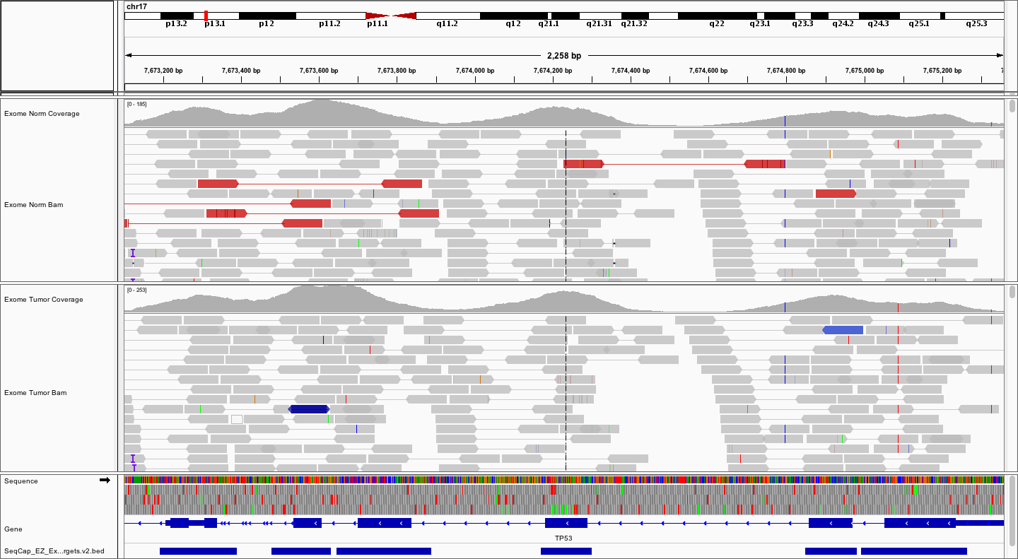
How does the coverage pattern compare to the coordinates of targeted regions?
Answer
As expected, the targeted regions closely overlap the coding exons.
Load the WGS BAMs
Lets start a new session and load the WGS BAMs, your URLs should look like these:
- http://s#.pmbio.org/align/WGS_Norm_merged_sorted_mrkdup_bqsr.bam
- http://s#.pmbio.org/align/WGS_Tumor_merged_sorted_mrkdup_bqsr.bam
Using the URLs above:
- If IGV is already running, start a new session with
File->New Session - Load the bam files (using the URLs above) with
File->Load from URL - Rename the tracks (e.g., WGS Norm Coverage, WGS Norm BAM, WGS Tumor Coverage, WGS Tumor BAM) by right-clicking on each track and selecting
Rename Track - Save session with
File->Save Session
View WGS alignments for an example gene
Once again, let’s take a look at TP53 on chr17. Simply type TP53 into the search box and hit Go or enter.
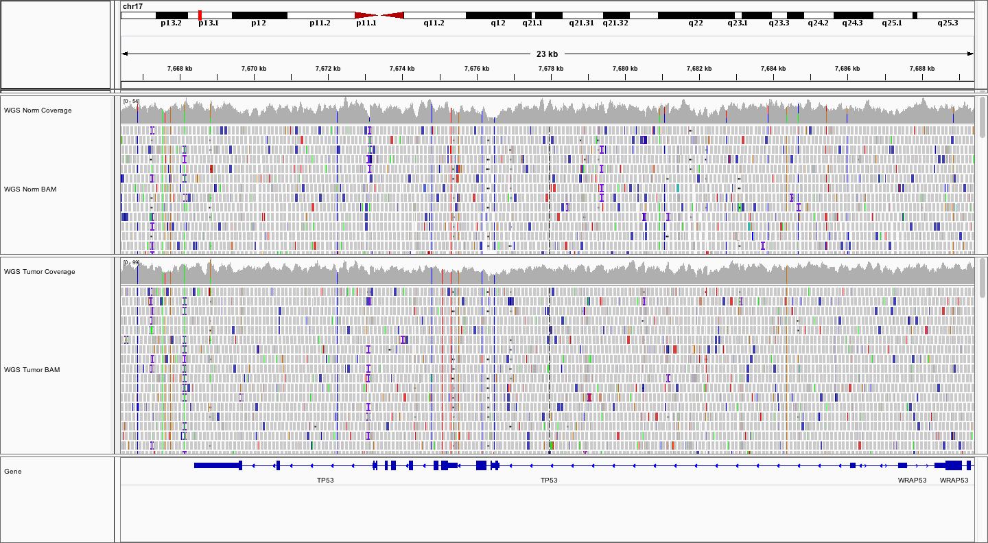
What does the average WGS coverage look like for Normal and Tumor? How does it differ from the exome coverage pattern? What about the fragment sizes?
Answer
The WGS Normal sample appears to have average coverage of ~50X whereas the normal has average coverage of ~75X. In general the fragment sizes seem a little larger, with a wider range, from ~250bp to ~600
Color alignments by library or read group by right-clicking on each alignment data track and selecting Color alignments by -> library or Color alignments by -> read group. How many read groups and libraries are there?
Answer
There were three libraries sequenced across 5 lanes. Lane has been used as read group in this case
Explore on your own
Spend some time scrolling around and zooming in and out to get a feel for the WGS data.
- Can you find any regions of low coverage? What are they correlated with?
- What is different between the variant allele fractions of the normal and tumor? What could explain this?
- What else of interest can you find?