RNAseq Fusion Filtering/Annotation/Review
Introduction
Pizzly generates outputs in .fasta and .json formats. Some initial filtering is performed automatically in pizzly, for example removing alignments where the distance of the breakpoint to exon boundaries is 10 or more base pairs. These automatically filtered reads are included in the outputs with unfiltered. suffix. In this module we will perform additional annotation, filtering and visualization of the .json output.
Annotation
JSON data (JavaScript Object Notation) are name/value pairs separated by a colon. Pairs are organized into objects within curly braces and arrays within square brackets. JSON data can be reorganized into tabular form in a delimited text file using many tools and programming languages. Below, we will use R and a modified script from the grolar GitHub repository by Matthew Bashton to annotate pizzly output and create a tabular, annotated output.
# Get R scripts for later use
cd /workspace/rnaseq/fusion
wget https://raw.githubusercontent.com/griffithlab/pmbio.org/master/assets/course_scripts/mod.grolar.R
wget https://raw.githubusercontent.com/griffithlab/pmbio.org/master/assets/course_scripts/import_Pizzly.R
# Open the R environment and set working directory
R
setwd("/workspace/rnaseq/fusion/")

# Install packages if necessary from these commented lines-
#  If asked about updating old packages (e.g. Old packages: 'MASS', 'devtools'... Update all/some/none? [a/s/n]:), select n
# install.packages("jsonlite")
# install.packages("dplyr")
# source("https://bioconductor.org/biocLite.R")
# biocLite()
# biocLite("ensembldb")
# biocLite("EnsDb.Hsapiens.v86")

# Load required packages
library(jsonlite)
library(dplyr)
library(EnsDb.Hsapiens.v86)
library(ggplot2))
edb = EnsDb.Hsapiens.v86

# Load data
suffix = "617.json"
JSON_files = list.files(path = "/workspace/rnaseq/fusion", pattern = paste0("*",suffix))
Ids = gsub(suffix, "", JSON_files)

# Load grolar.R script and run the GetFusionz_and_namez function to annotate
source("./mod.grolar.R")

# The function is too long to type out line by line, but we can view it by calling it without variables
GetFusionz_and_namez
#  Look through the funciton steps to get a sense of how our output is being processed.

# Run annotation script on each file in /workspace/rna/fusion suffixed with fusion.json
lapply(Ids, function(x) GetFusionz_and_namez(x, suffix=suffix))
The function should return:
[[1]]
[1] TRUE

[[2]]
[1] TRUE
Filtering
- The GetFusionz_and_namez script wrote two new files into /workspace/rnaseq/fusion:
norm-fuse_fusions_filt_sorted.txtandtumor-fuse_fusions_filt_sorted.txt. Let’s read those back into R and filter further:normal=read.table("./norm-fuse_fusions_filt_sorted.txt", header=T) tumor=read.table("./tumor-fuse_fusions_filt_sorted.txt", header=T) names(normal) - In addition to values present in the orignial
.jsonfiles, each fusion now has a unique identifier, sequence positions, and distance values for genes from the same chromosome:
> names(normal)
 [1] "ID"                   "paircount"            "splitcount"
 [4] "geneA.id"             "geneA.name"           "geneA.seq_name"
 [7] "geneA.gene_seq_start" "geneA.gene_seq_end"   "geneA.seq_strand"
[10] "geneB.id"             "geneB.name"           "geneB.seq_name"
[13] "geneB.gene_seq_start" "geneB.gene_seq_end"   "geneB.seq_strand"
[16] "same_chr"             "gene_distance"
- Common filtering tasks for fusion output include removing fusions from the tumor sample which are present in the normal, and removing fusions for which the is little support by pair and split read counts:
normal$genepr=paste0(normal$geneA.name,".",normal$geneB.name)
tumor$genepr=paste0(tumor$geneA.name,".",tumor$geneB.name)
uniqueTumor=subset(tumor, !(tumor$genepr %in% normal$genepr))
nrow(uniqueTumor)==nrow(tumor)
[1] FALSE
nrow(tumor)-nrow(uniqueTumor)
[1] 2
# There are two fusions (or at least fusion gene pairs) from the normal sample which are also present in the tumor.
# Examine the output of-
shared_src_tumor=subset(tumor, (tumor$genepr %in% normal$genepr))
shared_src_normal=subset(normal, (normal$genepr %in% tumor$genepr))
shared_src_tumor
shared_src_normal
- Filtering by counts:
# Merge normal and tumor data
normal$sample="normal"
tumor$sample="tumor"
allfusions=rbind(normal,tumor)
# Compare counts of paired and split reads
tapply(allfusions$paircount, allfusions$sample, summary)
$normal
   Min. 1st Qu.  Median    Mean 3rd Qu.    Max.
  0.000   0.000   0.000   1.148   2.000  24.000

$tumor
   Min. 1st Qu.  Median    Mean 3rd Qu.    Max.
 0.0000  0.0000  0.0000  0.5965  1.0000  6.0000

tapply(allfusions$splitcount, allfusions$sample, summary)
$normal
   Min. 1st Qu.  Median    Mean 3rd Qu.    Max.
  0.000   1.000   1.000   4.901   3.000 123.000

$tumor
   Min. 1st Qu.  Median    Mean 3rd Qu.    Max.
  0.000   1.000   1.000   2.526   3.000  24.000
# As a density plot
countplot=list()
countplot[[1]]=ggplot(allfusions, aes(paircount, fill=sample))+geom_density(alpha=.4)+geom_vline(xintercept=2)+coord_fixed(ratio=15)
countplot[[2]]=ggplot(allfusions, aes(splitcount, fill=sample))+geom_density(alpha=.4)+coord_cartesian(ylim= c(0,.2))+geom_vline(xintercept=5)+coord_fixed(ratio=200)
pdf("countplot.pdf")
countplot
dev.off()
- Results should look like this:
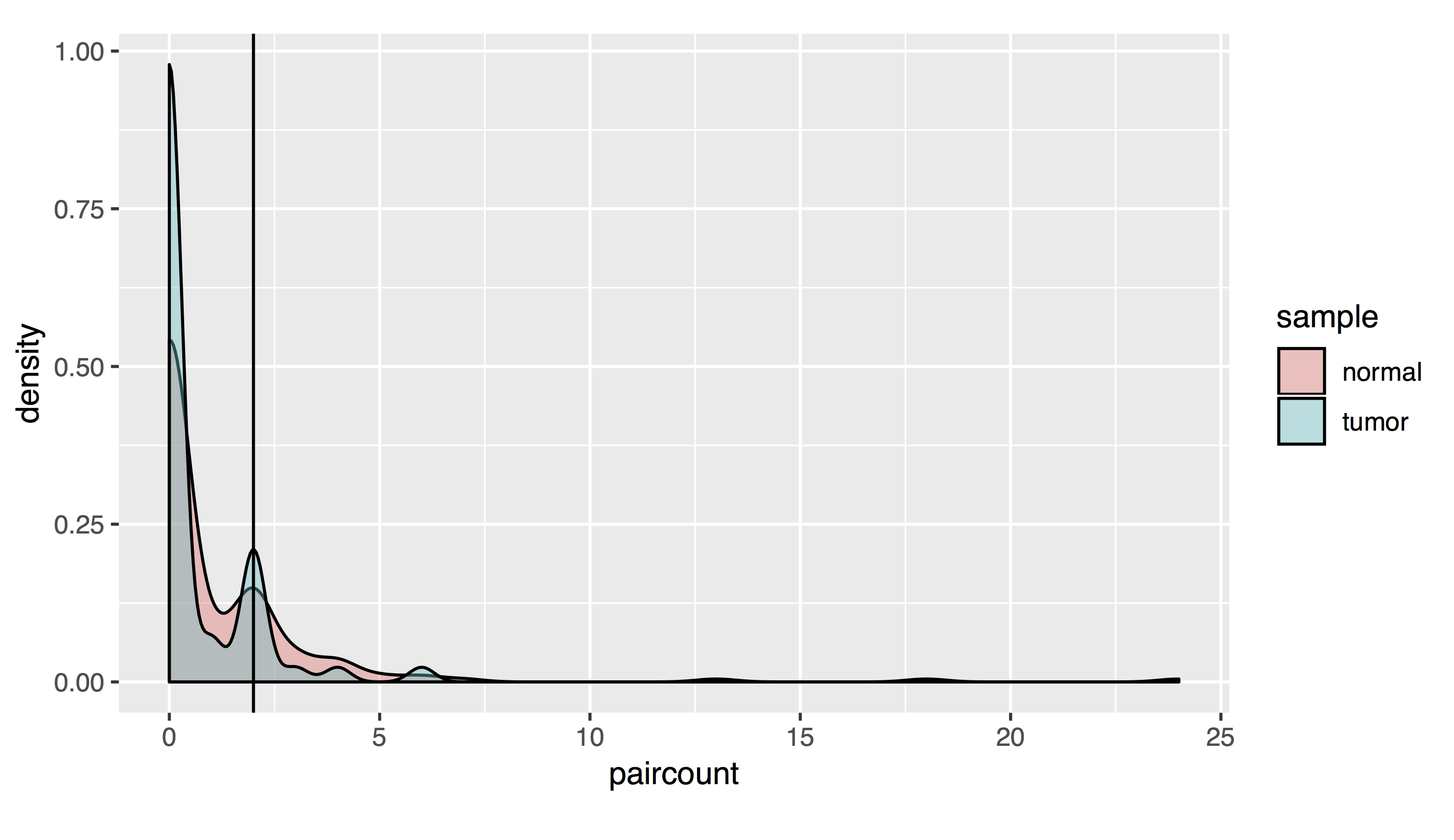
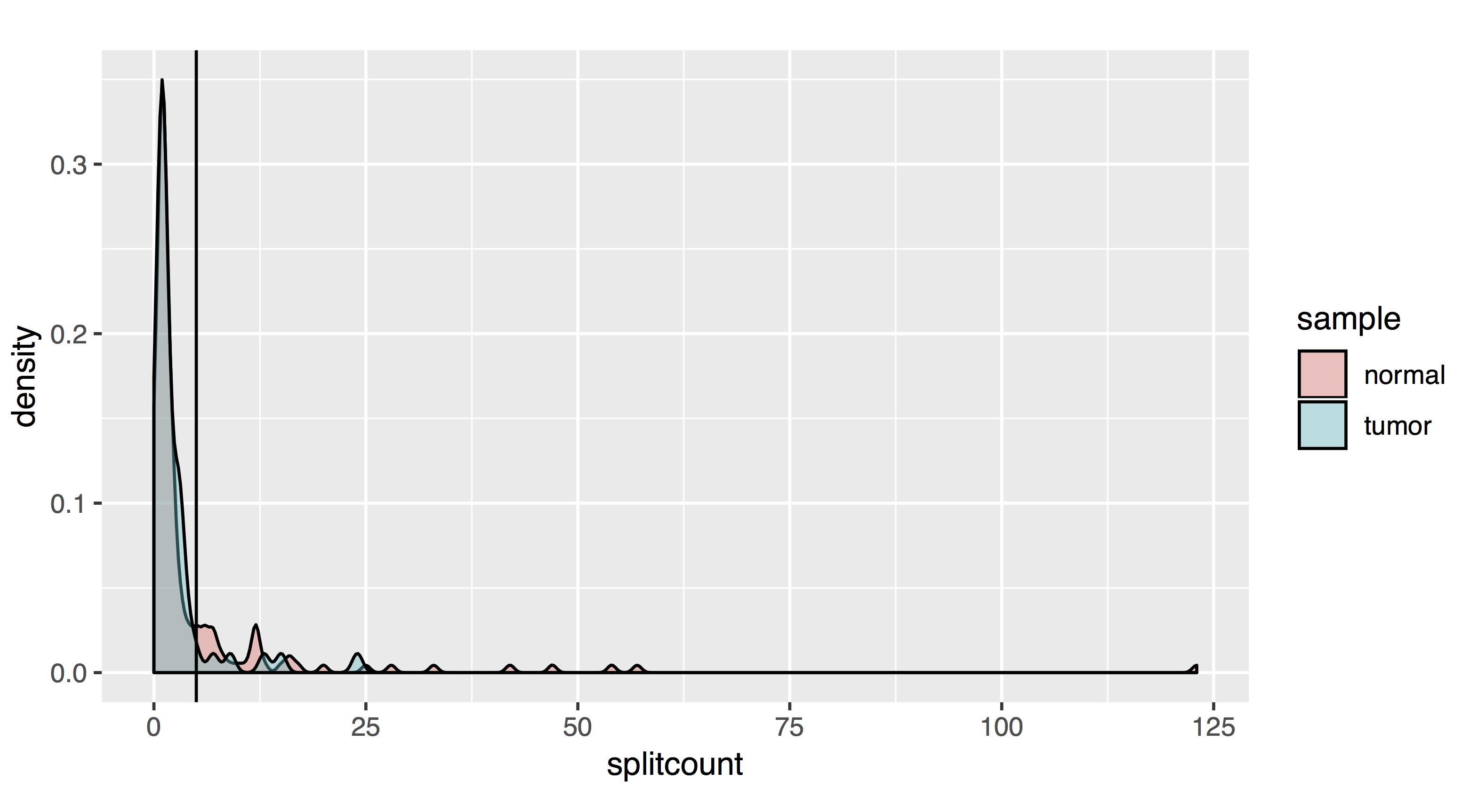
To filter, let’s take all fusions with a pair read count of at least 2 and a split read count of at least 5:
nrow(allfusions)
[1] 239
allfusions=allfusions[which(allfusions$paircount >= 2 & allfusions$splitcount >= 5),]
nrow(allfusions)
[1] 27
write.table(allfusions, "allfusions.txt")
Visualization:
Chimeraviz is an R package for visualizing fusions from RNA-seq data. The chimeraviz package has import functions built in for a variety of fusion-finder programs, but not for pizzly. We will have to load our own import function that you downloaded above:
# Enter R, install and load chimeraviz
R
source("https://bioconductor.org/biocLite.R")
biocLite("chimeraviz")
# (if asked to update old packages, you can ignore- Update all/some/none? [a/s/n]:)
library(chimeraviz)
# Use the pizzly importer script to import fusion data
source("./import_Pizzly.R")
# You can view the function by calling it without variables
importPizzly
fusions = importPizzly("./allfusions.txt","hg38")
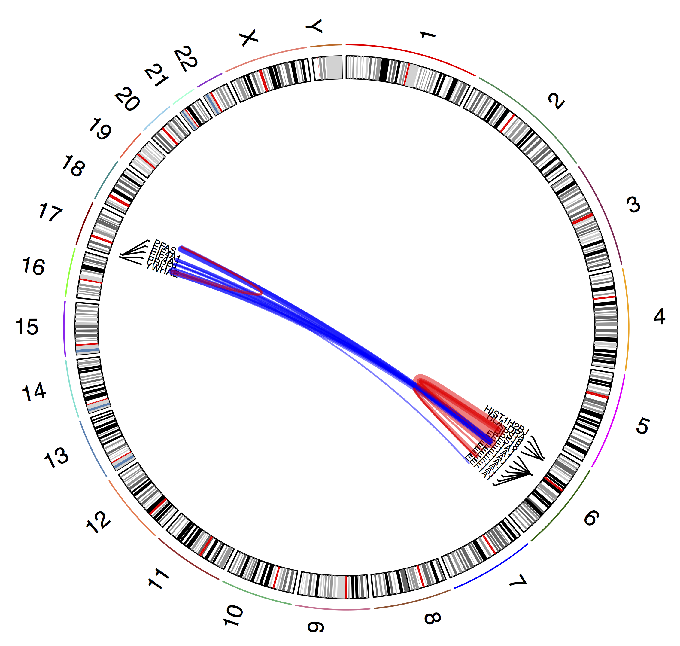
pdf("chr617-fuse-circ.pdf")
plot_circle(fusions)
dev.off()
The resulting circos plot shows our filtered gene fusions (blue for inter-chromosomal and red for intra-chromosomal)