ChIP-seq analysis
ChIP-seq analysis
This exercise uses H3K4me3 ChIPseq data from the brain tissue of a Alzheimer’s disease patient that was produced by the ENCODE consortium (accession ENCBS748EGF) First, click through to that ENCODE page and compare it to another H3K4me3 experiment on the portal: ENCSR539TKY
Notice that ENCODE enforces rigorous QC standards and displays that information prominently on their page. When analyzing your own ChIP-seq data, their data quality standards are a great benchmark to use. This lesson doesn’t cover doing ChIP-seq QC, but it’s incredibly important, given that ChIP-seq experiments are more finicky than many other sequencing approaches. There are many resources available for more information, including the excellent Intro to ChIPseq using HPC online course.
To get started with analyzing this data, start by making a directory where we will do the analysis.
mkdir -p ~/workspace/chipseq_data
cd ~/workspace/chipseq_data
We will use a bash script to download and organize the data. Bash scripts allow us to take commands we would run in the command line and combine them into a single script so that we can execute them easily. After downloading the script, explore it using the less command.
wget https://raw.githubusercontent.com/ksinghal28/pmbio.org/master/assets/course_scripts/download_and_organize_chipseq_data.sh
less download_and_organize_chipseq_data.sh
The bash script downloads the tar file containing the pre-aligned BAM files, untars it, moves some files and cleans up the contents.
Try running the script and use ls to see the files that are generated.
bash download_and_organize_chipseq_data.sh
ls
These are small bam files that have been subset to just the first 10Mb of chr17 to speed up this analysis.
In order for tools to access the data in these bams, you’ll need to create an index file for each. Instead of running that command 4 different times, use xargs and then use ls to check if the index files were generated:
ls -1 *.bam | xargs -n 1 samtools index
ls
Neat! But how did that work?
ls -1 *.bam lists all files ending with the .bam extension, with the -1 part ensuring they go to their own line.
xargs or ‘extended arguments’ allows us to build and execute commands from the standard input. Here, it helps us take the files output from ls -1 *.bam and use that as an input to samtools index. The -n 1 argument ensures that each file is considered separately.
Here’s a toy example comparing how xargs works for counting lines in a BAM file and changing the -n argument-
ls -1 *.bam | xargs -n 1 wc -l
ls -1 *.bam | xargs -n 2 wc -l
ls -1 *.bam | xargs -n 3 wc -l
ls -1 *.bam | xargs -n 4 wc -l
Calling peaks
MACS is a package for ChIP-seq analysis that has many utilities. Instead of using a pre-installed version of this software, we will take advantage of a docker container made by the authors of the package. You can see the utilities in MACS for yourself by running-
docker run fooliu/macs2 --help
Today, we’re interested in using the callpeak utility to find peaks in our ChIP-seq data that correspond to H3K4me3 marks in this sample. Let’s see what inputs are needed:
docker run fooliu/macs2 callpeak --help
Woah, that’s a lot of options. MACS is highly configurable, and different types of ChIP-seq experiments might require different tweaks. Luckily for you, it has sensible defaults that will work well for the data type that you’re exploring today.
One step that’s frequently done in ChIP-seq is the removal of duplicate reads. In the MACS options below, there are some for handling dups appropriately, but we need to know what we’re dealing with first. Thanks to the Explain Sam Flags site, we know that duplicate reads have a flag of 1024 set. Let’s check this bam file for duplicate reads:
samtools view -f 1024 alz_H3K4me3_rep1.bam | wc -l
Looks like they removed the duplicate reads already as part of their filtering process. Creating a new bam sans duplicates is typically not necessary, but since they have done it, we won’t need to worry about dealing with them in MACS.
As your next step, go ahead and try running MACS on this data. Note that you’re providing the ChIP data along with “input” data that serves as background. Having such input data is essential to distinguishing true signal from noise.
docker run -v /home/ubuntu/workspace/chipseq_data:/home/ubuntu/workspace/chipseq_data fooliu/macs2 callpeak -t /home/ubuntu/workspace/chipseq_data/alz_H3K4me3_rep1.bam /home/ubuntu/workspace/chipseq_data/alz_H3K4me3_rep2.bam -c /home/ubuntu/workspace/chipseq_data/alz_input_rep1.bam /home/ubuntu/workspace/chipseq_data/alz_input_rep2.bam -f BAM --call-summits -p 0.01 -n /home/ubuntu/workspace/chipseq_data/macs_callpeak
MACS outputs
MACS creates outputs in several different formats that can be useful in different contexts:
macs_callpeak_peaks.narrowPeaka modified bed format that includes information about the coordinates, size and significance of each peak:
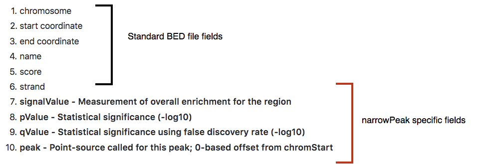
(image from https://hbctraining.github.io/Intro-to-ChIPseq/lessons/05_peak_calling_macs.html CC-N)
-
macs_callpeak_summits.bedeach peak can contain one or more “summits” that mark a local maximum. This bed file contains these locations. -
macs_callpeak_peaks.xlsDespite the extension, this is not an Excel file. Take a look at it usingless. The metadata in header contains information on exactly how MACS was run and a detailed report on the parameters that MACS learned from the data. The data in the body contains every peak and summit along with information on significance and such, mirroring some of the information in the other two files. -
macs_callpeak_model.rMACS outputs an R script that can be used to generate a plot.
Go ahead and generate that plot now:
Rscript macs_callpeak_model.r
In an ideal case, the pdf file that it creates will look something like this, representing the bimodal pattern of the shift size.
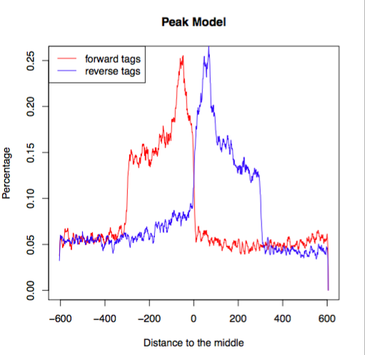 (image from https://hbctraining.github.io/Intro-to-ChIPseq/lessons/05_peak_calling_macs.html)
In this case, since we’re using a small subset of the genome, the data is sparse and a little more choppy, but you can see the same essential shape.
Manual review
ChIP-seq library preparation is notoriously finicky and it’s important to dig into the raw data and really get a feel for how it looks before believing that your results are solid. IGV is great for this, but it’s rather hard to load up 4 bam files to review on a laptop screen (and it certainly doesn’t scale to experiments with a dozen or more samples!). Since the essential feature that we care about with ChIP-seq is the read depth, we can use a format more suited to that: bigwig. The example command below is how you can run it on 1 BAM file, but instead of running it once for each BAM file, we can run it all together in 1 for loop!
#example command
#docker run -v /home/ubuntu/workspace:/docker_workspace quay.io/wtsicgp/cgpbigwig:1.6.0 bam2bw -a -r /docker_workspace/ensembl-vep/homo_sapiens/108_GRCh38/Homo_sapiens.GRCh38.dna.toplevel.fa.gz -i /docker_workspace/chipseq_data/alz_H3K4me3_rep1.bam -o /docker_workspace/chipseq_data/alz_H3K4me3_rep1.bw

#using a for loop instead
for i in *.bam;do
  echo "converting file $i"
  docker run -v /home/ubuntu/workspace:/docker_workspace quay.io/wtsicgp/cgpbigwig:1.6.0 bam2bw -a -r /docker_workspace/ensembl-vep/homo_sapiens/108_GRCh38/Homo_sapiens.GRCh38.dna.toplevel.fa.gz -i /docker_workspace/chipseq_data/$i -o /docker_workspace/chipseq_data/$(basename $i .bam).bw
done
A bigwig file is a compressed format that contains genomic coordinates and values associated with each. In this case, it will be depth over the entire genome. It’s important to remember that when making peak calls, MACS isn’t using the raw depth, but is applying normalization to the data. Nonetheless, this is often a reasonable way to examine the data, especially when the experiments are similar in terms of depth and quality.
Exercises:
- Open IGV and load your 4 bigwig files.
- Open IGV and load one of your bam files. Compare the information in the bigwig to that contained in the bam. Remove the bam and coverage tracks when you’re done.
- Give the input controls and H3K4me3 tracks different colors to make them easy to distinguish at a glance.
- Load your narrowPeaks file into IGV.
- Navigate to chr17:1-100 (all of this data is on chr17), then click on the narrowPeaks track and hit
CTRL-Fto jump to the first peak. How’s it look? - It’s awfully hard to interpret these peak heights when they’re all being scaled differently. Set them to be the same height by selecting them (shift+click), then right click and enable “Group Autoscale”
- Flip through a few peaks - do they seem believable compared to the surrounding background data and input tracks?
- Scroll a little bit away from one of the peaks. What happens to the autoscaled tracks? How does the data look out here?
- Jump to the WRAP53 gene and take a look at the peak in the middle. Group autoscale hides what’s going on - how can you tweak things to look more visible? Do you believe that this is a solid peak call?
- This is an exceptionally clean experiment and the peaks generally look great, but in less clear cases, you might want to do additional filtering. To adjust the stringency of these calls, go back to the narrowPeaks file and filter it to only include calls that exceed a -log10(pvalue) of 10. Here’s an example of using awk to filter a tab-separated file on the first column of a file - adapt it to your needs.
awk '{if($1>5){print $0}}' infile >outfile'
-
Save the result as another narrowPeaks file and load it in IGV.
-
How could we use command line set operations to make a narrowPeaks file that contained only the lines that were removed?