Data munging / cleaning
Adapted from the NCEAS dataviz module and R for Data Science
Introduction
Learning outcomes
Students should
- Learn what it means to examine and clean their data
- Learn how to reshape and restructure their data with base R and dplyr functions
- Pull out informative subsets of a dataset to make an attractive figure
Lesson
Let’s look at an example dataset (one we’ve made) and go over some ways we might QA/QC this dataset.
It is an arbitrary temperature study with six sites. Within each site, there are 6 plots and we took 10 samples of temperature (degrees C) per plot.
Step one: Import and prepare
fundata <- read.csv("http://genomedata.org/seq-tec-workshop/misc/fundata.csv")
head(fundata) # Look at the data
##   siteplot       date temp_c
## 1      A.1 03-21-2017  31.50
## 2      B.2 04-21-2017  33.63
## 3      C.3 05-21-2017  32.56
## 4      D.4 06-21-2017  31.22
## 5      E.5 07-21-2017  25.44
## 6      F.6 08-21-2017  33.55
str(fundata)
## 'data.frame':    355 obs. of  3 variables:
##  $ siteplot: chr  "A.1" "B.2" "C.3" "D.4" ...
##  $ date    : chr  "03-21-2017" "04-21-2017" "05-21-2017" "06-21-2017" ...
##  $ temp_c  : num  31.5 33.6 32.6 31.2 25.4 ...
summary(fundata)
##    siteplot             date               temp_c
##  Length:355         Length:355         Min.   :-9999.00
##  Class :character   Class :character   1st Qu.:   26.75
##  Mode  :character   Mode  :character   Median :   30.20
##                                        Mean   : -111.25
##                                        3rd Qu.:   33.36
##                                        Max.   :  180.00
##                                        NA's   :1
What’s our assessment of this dataset from the above commands?
- The site and plot codes are smushed together in one column.
- The dates look a bit funky. What format is that?
- The range on the temperatures surely can’t be right
Split siteplot into two columns
Here’s some example code showing how to generate a dataframe with ugly smashed together variables. and then how to split it out:
library(tidyverse)
lettersdf <- data.frame(letters = paste(LETTERS, rev(LETTERS), sep = "."))
head(lettersdf)
##   letters
## 1     A.Z
## 2     B.Y
## 3     C.X
## 4     D.W
## 5     E.V
## 6     F.U
separate(lettersdf,letters, c("letter_one", "letter_two"), sep = "\\.")
##    letter_one letter_two
## 1           A          Z
## 2           B          Y
## 3           C          X
## 4           D          W
## 5           E          V
## 6           F          U
## 7           G          T
## 8           H          S
## 9           I          R
## 10          J          Q
## 11          K          P
## 12          L          O
## 13          M          N
## 14          N          M
## 15          O          L
## 16          P          K
## 17          Q          J
## 18          R          I
## 19          S          H
## 20          T          G
## 21          U          F
## 22          V          E
## 23          W          D
## 24          X          C
## 25          Y          B
## 26          Z          A
Exercise: Using your fundata object,split the siteplot column into
two columns called site and plot:
Convert the dates to real R dates
These dates use a format that isn’t wrong, but isn’t ideal for plotting and such. What happens when we try to sort them?
head(sort(fundata$date))
## [1] "03-21-2016" "03-21-2017" "03-21-2017" "03-21-2017"
## [5] "03-21-2017" "03-21-2017"
Ugh - these are characters, and so it’s not sorting how we might expect.
When you have dates in R, it’s usually best to convert them to a Date
object. The function we’ll use is as.Date. Here’s an example of using
it on a few dates:
datestrings <- c("2000-08-03", "2017-02-20", "1980-04-27")
class(datestrings)
## [1] "character"
mydate <- as.Date(datestrings, format = "%Y-%m-%d")
mydate
## [1] "2000-08-03" "2017-02-20" "1980-04-27"
class(mydate)
## [1] "Date"
Exercise: Convert the date column in fundata to from a character
vector to a Date vector with as.Date():
Step two: Checking assumptions in the data
site and plot columns
Let’s start by looking at the site column for potential issues.
The table function is a great way to tally the occurrences of each of
the unique values in a vector:
table(c("A", "A", "B", "C"))
##
## A B C
## 2 1 1
fish <- c("gag grouper", "striped bass", "red drum", "gag grouper")
table(fish)
## fish
##  gag grouper     red drum striped bass
##            2            1            1
To ahead and apply table to the site column. Based on our
experimental design, we expect to see 60 observations from each site. Do
we?
We can see we’re missing some observations from A, C, and E. Depending on our needs, we may need to go back to our field notes to find out what happened.
temp_c column
Get some basic stats about the temp_c column with summary:
summary(fundata$temp_c)
##     Min.  1st Qu.   Median     Mean  3rd Qu.     Max.     NA's
## -9999.00    26.75    30.20  -111.25    33.36   180.00        1
Or look directly at the range of values with range:
range(fundata$temp_c)
## [1] NA NA
Plotting your data is always a good idea and we can often find new insights or issues this way. For univariate data, a box plot is a great way to look at the distribution of values:
boxplot(rnorm(100, 50, 5))
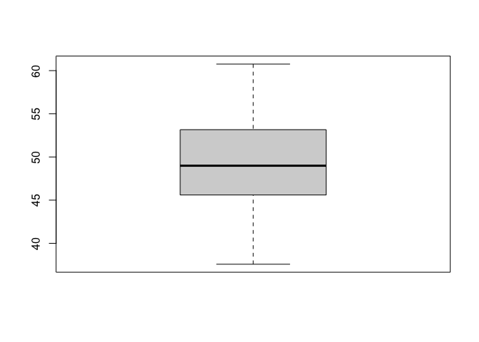
Exercise Use the boxplot() function to make a boxplot of the
temperature values
Those outlier values can’t be right! Before we move on, let’s fix the -9999 and 180 observations by removing them.
Exercise: Remove the rows with temperatures of -9999 and 180:
Oh no, not only do we have weird data, we also have missing data:
any(is.na(fundata$temp_c))
## [1] TRUE
“NA” is its own type in R.
is.na(2)
## [1] FALSE
is.na(NA)
## [1] TRUE
is.na(c(1, NA, 3))
## [1] FALSE TRUE FALSE
fish <- c("gag grouper", NA, "red drum", NA)
fish
## [1] "gag grouper" NA "red drum" NA
# Filter NAs in a character vector
fish[!is.na(fish)]
## [1] "gag grouper" "red drum"
# Remember we can subset the rows in a data.frame like:
fundata[c(1, 2, 3),] # First, second, third rows
##   siteplot       date temp_c
## 1      A.1 03-21-2017  31.50
## 2      B.2 04-21-2017  33.63
## 3      C.3 05-21-2017  32.56
#or
fundata[which(fundata$site == "A"),] # Just the rows with site == "A"
## [1] siteplot date     temp_c
## <0 rows> (or 0-length row.names)
# Write an expression using `is.na` to subset fundata and save the result
# Your code here:
# e.g. fundata$site <-
Your experimental design may dictate the way you handle missing data, but today, we’re just going to remove those rows.
Exercise Write an expression using is.na to subset fundata,
removing rows with missing temperature values and save the result
Manipulating data with dplyr
The dplyr package contains lots of useful functions for manipulating
data.
Let’s try it with the starwars data set. As a first step, let’s look
at what’s in this:
starwars
## # A tibble: 87 × 14
## name height mass hair_…¹ skin_…² eye_c…³ birth…⁴ sex
## <chr> <int> <dbl> <chr> <chr> <chr> <dbl> <chr>
## 1 Luke Skyw… 172 77 blond fair blue 19 male
## 2 C-3PO 167 75 <NA> gold yellow 112 none
## 3 R2-D2 96 32 <NA> white,… red 33 none
## 4 Darth Vad… 202 136 none white yellow 41.9 male
## 5 Leia Orga… 150 49 brown light brown 19 fema…
## 6 Owen Lars 178 120 brown,… light blue 52 male
## 7 Beru Whit… 165 75 brown light blue 47 fema…
## 8 R5-D4 97 32 <NA> white,… red NA none
## 9 Biggs Dar… 183 84 black light brown 24 male
## 10 Obi-Wan K… 182 77 auburn… fair blue-g… 57 male
## # … with 77 more rows, 6 more variables: gender <chr>,
## # homeworld <chr>, species <chr>, films <list>,
## # vehicles <list>, starships <list>, and abbreviated variable
## # names ¹hair_color, ²skin_color, ³eye_color, ⁴birth_year
## # ℹ Use `print(n = ...)` to see more rows, and `colnames()` to see all variable names
Notice that this output doesn’t look exactly like our fundata data
frame. It’s stored in something called a “tibble”. The details are
largely beyond this course, but thinking of it as a “fancy data frame”
is pretty much right on.
We can use base R functions format for interfacing with this data:
You can access a single element:
starwars[3,2]
## # A tibble: 1 × 1
##   height
##    <int>
## 1     96
or filter the data to only characters that have light skin and brown eyes:
starwars[starwars$skin_color == "light" & starwars$eye_color == "brown", ]
## # A tibble: 7 × 14
## name height mass hair_…¹ skin_…² eye_c…³ birth…⁴ sex
## <chr> <int> <dbl> <chr> <chr> <chr> <dbl> <chr>
## 1 Leia Organa 150 49 brown light brown 19 fema…
## 2 Biggs Dark… 183 84 black light brown 24 male
## 3 Cordé 157 NA brown light brown NA fema…
## 4 Dormé 165 NA brown light brown NA fema…
## 5 Raymus Ant… 188 79 brown light brown NA male
## 6 Poe Dameron NA NA brown light brown NA male
## 7 Padmé Amid… 165 45 brown light brown 46 fema…
## # … with 6 more variables: gender <chr>, homeworld <chr>,
## # species <chr>, films <list>, vehicles <list>,
## # starships <list>, and abbreviated variable names
## # ¹hair_color, ²skin_color, ³eye_color, ⁴birth_year
## # ℹ Use `colnames()` to see all variable names
Filter rows with filter()
dplyr gives us some new fancy tools to slice and dice this data any
way we want, and also introduces a new way to move data around with
pipes.
To achieve the same filter as above, we can use this command:
starwars %>% filter(skin_color == "light", eye_color == "brown")
## # A tibble: 7 × 14
## name height mass hair_…¹ skin_…² eye_c…³ birth…⁴ sex
## <chr> <int> <dbl> <chr> <chr> <chr> <dbl> <chr>
## 1 Leia Organa 150 49 brown light brown 19 fema…
## 2 Biggs Dark… 183 84 black light brown 24 male
## 3 Cordé 157 NA brown light brown NA fema…
## 4 Dormé 165 NA brown light brown NA fema…
## 5 Raymus Ant… 188 79 brown light brown NA male
## 6 Poe Dameron NA NA brown light brown NA male
## 7 Padmé Amid… 165 45 brown light brown 46 fema…
## # … with 6 more variables: gender <chr>, homeworld <chr>,
## # species <chr>, films <list>, vehicles <list>,
## # starships <list>, and abbreviated variable names
## # ¹hair_color, ²skin_color, ³eye_color, ⁴birth_year
## # ℹ Use `colnames()` to see all variable names
These work the same as unix pipes - data flows from left to right. We
took the data contained in starwars and piped into the filter function
and told it which columns to operate on. This is in some ways a little
more intuitive and easier to type than the above
Arrange rows with arrange()
We can also reorder or sort data:
starwars %>% arrange(height, mass)
## # A tibble: 87 × 14
## name height mass hair_…¹ skin_…² eye_c…³ birth…⁴ sex
## <chr> <int> <dbl> <chr> <chr> <chr> <dbl> <chr>
## 1 Yoda 66 17 white green brown 896 male
## 2 Ratts Tye… 79 15 none grey, … unknown NA male
## 3 Wicket Sy… 88 20 brown brown brown 8 male
## 4 Dud Bolt 94 45 none blue, … yellow NA male
## 5 R2-D2 96 32 <NA> white,… red 33 none
## 6 R4-P17 96 NA none silver… red, b… NA none
## 7 R5-D4 97 32 <NA> white,… red NA none
## 8 Sebulba 112 40 none grey, … orange NA male
## 9 Gasgano 122 NA none white,… black NA male
## 10 Watto 137 NA black blue, … yellow NA male
## # … with 77 more rows, 6 more variables: gender <chr>,
## # homeworld <chr>, species <chr>, films <list>,
## # vehicles <list>, starships <list>, and abbreviated variable
## # names ¹hair_color, ²skin_color, ³eye_color, ⁴birth_year
## # ℹ Use `print(n = ...)` to see more rows, and `colnames()` to see all variable names
If you provide more than one column name, each additional column will be used to break ties in the values of the preceding column.
Select columns with select()
This is kind of a big dataset with lots of columns, maybe we only really care about a few of them. Let’s grab just those:
starwars %>% select(hair_color, skin_color, eye_color)
## # A tibble: 87 × 3
##    hair_color    skin_color  eye_color
##    <chr>         <chr>       <chr>
##  1 blond         fair        blue
##  2 <NA>          gold        yellow
##  3 <NA>          white, blue red
##  4 none          white       yellow
##  5 brown         light       brown
##  6 brown, grey   light       blue
##  7 brown         light       blue
##  8 <NA>          white, red  red
##  9 black         light       brown
## 10 auburn, white fair        blue-gray
## # … with 77 more rows
## # ℹ Use `print(n = ...)` to see more rows
If you want to save the output of these filtering operations for use in later code, instead of just sending it to the screen, add a variable name:
mydata = starwars %>% select(hair_color, skin_color, eye_color)
Finally, we can chain together powerful expressions to group and summarize data:
starwars %>%
  group_by(species, sex) %>%
  select(height, mass) %>%
  summarize(
    height = mean(height, na.rm = TRUE),
    mass = mean(mass, na.rm = TRUE)
  )
## Adding missing grouping variables: `species`, `sex`
## `summarise()` has grouped output by 'species'. You can override
## using the `.groups` argument.

## # A tibble: 41 × 4
## # Groups:   species [38]
##    species   sex    height  mass
##    <chr>     <chr>   <dbl> <dbl>
##  1 Aleena    male      79   15
##  2 Besalisk  male     198  102
##  3 Cerean    male     198   82
##  4 Chagrian  male     196  NaN
##  5 Clawdite  female   168   55
##  6 Droid     none     131.  69.8
##  7 Dug       male     112   40
##  8 Ewok      male      88   20
##  9 Geonosian male     183   80
## 10 Gungan    male     209.  74
## # … with 31 more rows
## # ℹ Use `print(n = ...)` to see more rows
It takes time to really know these tools intuitively, but this gives you
a flavor of what you can do with it. There are many additional useful
functions like mutate(), gather() and spread() that are worth
exploring, but all of them should be used for the same purpose - to get
your data cleaned up and into a format that is useful for statistics or
plotting.
Exercise: Use ggplot to make a beautiful figure demonstrating the relationship between height, mass, and sex in these fictional starwars species. Remember axis labels, legends, themes, and other things that we talked about in the previous lesson!