Somatic SV Filtering/Annotation/Review
Now that we have our manta results, lets do some basic filtering annotation and visualization. First off Let’s go ahead and look at how many SVs were called and if they passed or failed filters. We can accomplish this by cutting out the 7th column in the vcf file.
cd /workspace/somatic/manta_wgs/results/variants
zcat somaticSV.vcf.gz | grep -v "^#" |cut -f 7 | sort | uniq -c
You should see something like this:
1 MaxMQ0Frac
1 MaxMQ0Frac;MinSomaticScore
29 MinSomaticScore
129 PASS
We can see that the majority of the SVs passed mantas default filters however 31 failed by either not meeting the min somatic score cutoff under mantas somatic model or the fraction of reads with a MAPQ0 (i.e. aligned to multiple locations) around the breakpoints of the SV exceeded the threshold. For a full explanation of why manta may have failed a somatic variant look at the manta documentation available here.
Manta will detect the following SV types:
- Insertions
- Deletions
- Inversions
- Tandem Duplications
- Interchromosomal Translocations
Lets do some command line magic to see the breakdown of SV types in our list with a bit of command line magic
zcat somaticSV.vcf.gz | grep -v "^#" | grep -iw "PASS" | cut -f 3 | tr ":" "\t" | cut -f 1 | sort | uniq -c
4 MantaBND
64 MantaDEL
39 MantaDUP
2 MantaINS
20 MantaINV
we can see from the output that we have 4 interchromosomal translocations, 64 deletions, 39 duplications, 2 insertions, and 20 inversions passing filters.
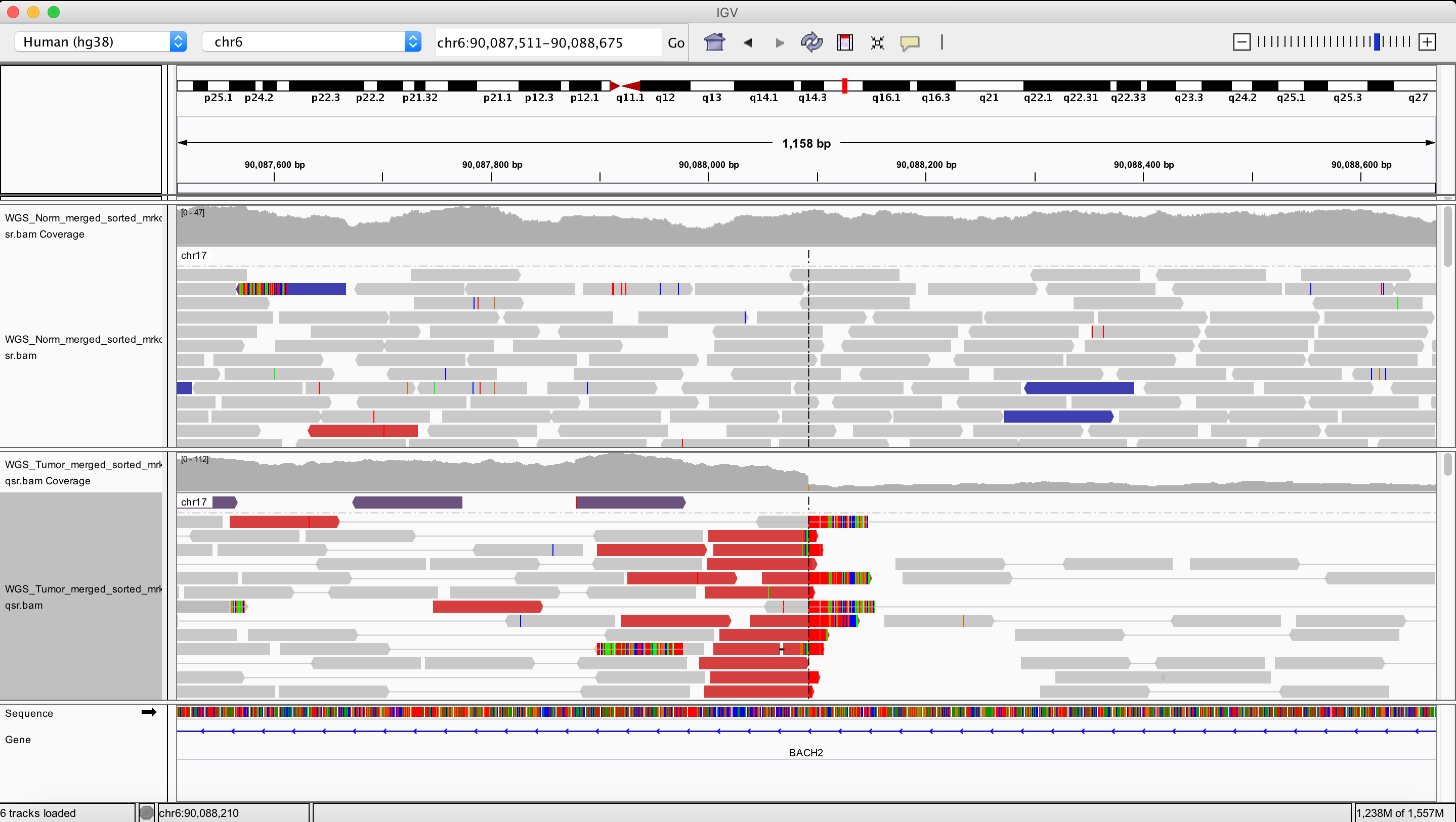
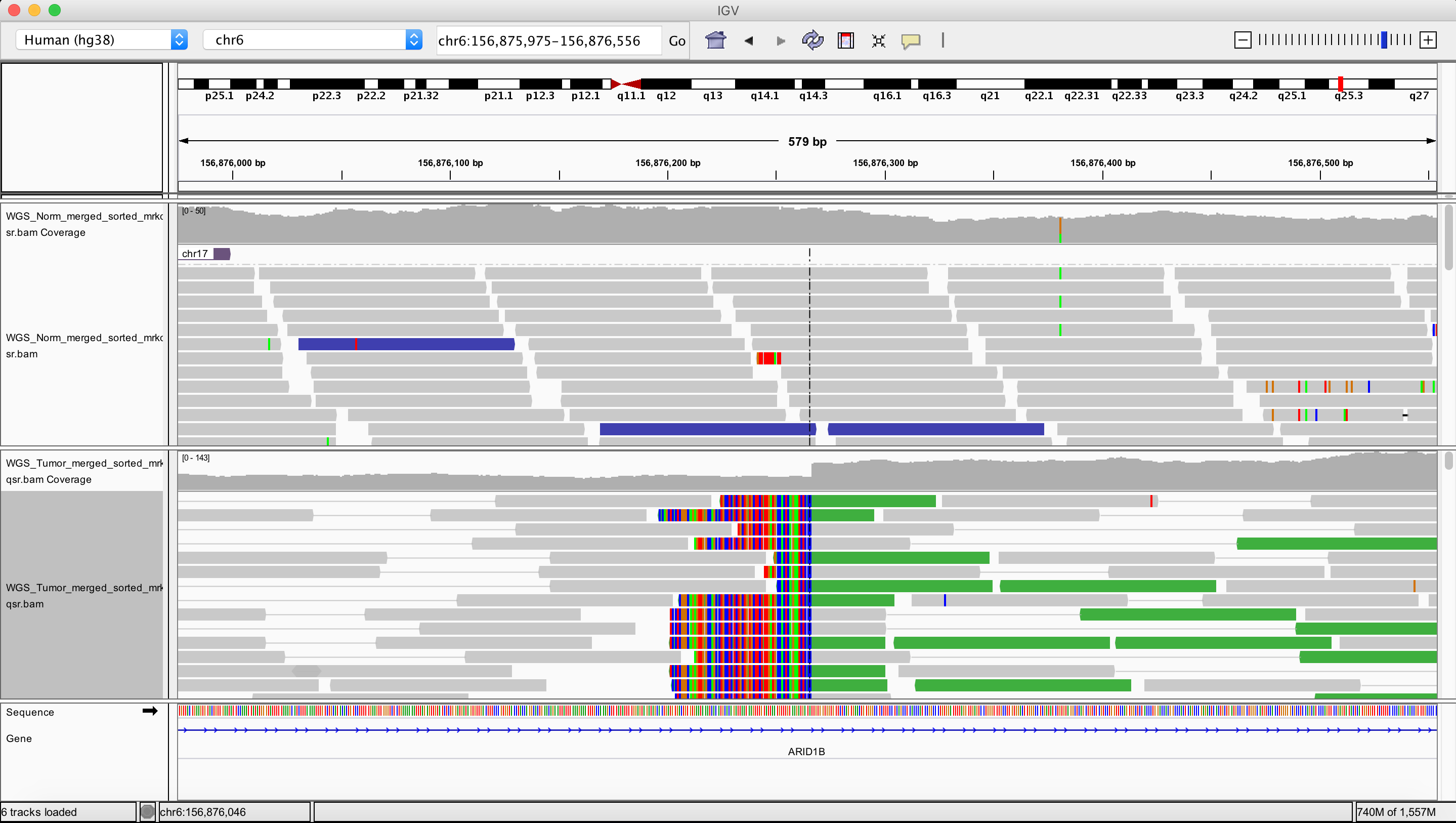
Let’s look at an example of each of these in IGV to evaluate them. As an aside IGV has some nice documentation on interpreting SVs by insert size and pair orientation here and here.
Interchromosomal translocation
chr6 695390
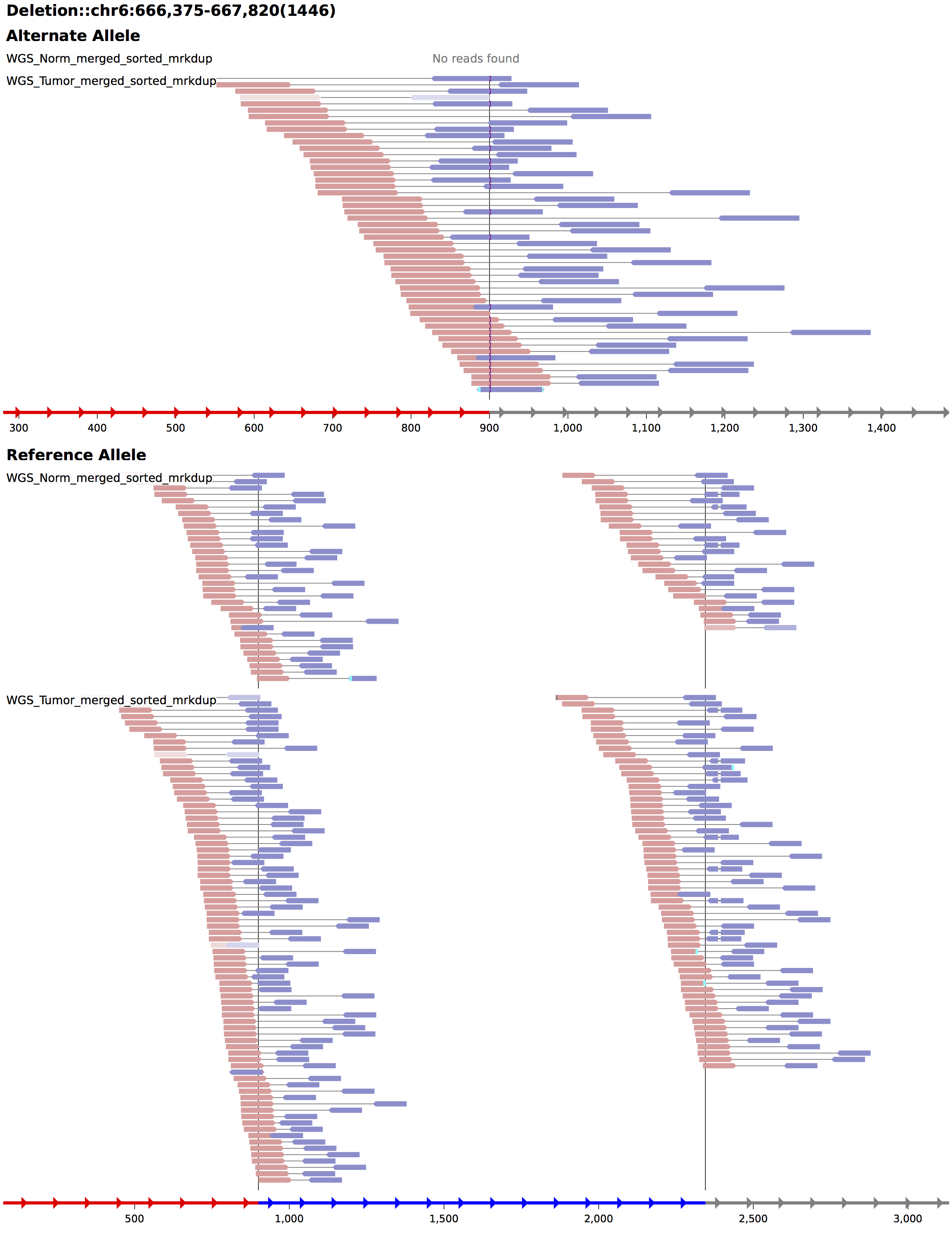
Deletion
chr6 90088092
Duplication
chr6 156876266
Inversion
chr6 86719474
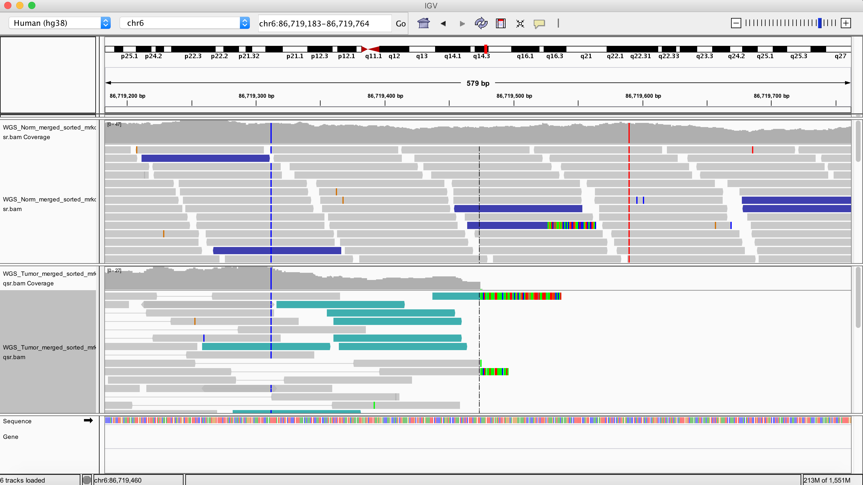
Visualizing with svviz
Use a docker image to run svviz2
# create a directory for the svviz2 results
cd /workspace/somatic/manta_wgs/results/variants/
mkdir svviz2

# create a filtered version of the SVs that removes large SVs that take a while to visualize (e.g. >2500 bases)
# note that some sizes are indicated as -ve values so we are using two regular expressions to grab just the number before assessing (SVLEN > 2500)
zcat somaticSV.vcf.gz | perl -ne 'if ($_ =~ /SVLEN\=\-(\d+)/){if ($1 > 2500){next;}} if ($_ =~ /SVLEN\=(\d+)/){if ($1 > 2500){next;}}print $_' > somaticSV.filtered.vcf

# use svviz2 within a docker image to produce visualiatons for our manta SV results
docker pull sridnona/svviz2:v2

# test the docker installation
docker run sridnona/svviz2:v2 /usr/local/bin/svviz2 --help

# start an interactive session with this docker image. make sure the /workspace volume is accessible inside the docker containers and mounted at the same path
docker run -i -v /workspace:/workspace -t sridnona/svviz2:v2 /bin/bash

# make sure we can run docker inside the container
svviz2 --help

# run svviz on the manta SV results, supplying the VCF, reference genome, normal WGS BAM, and tumor WGS BAM
svviz2 --ref /workspace/inputs/references/genome/ref_genome.fa --variants /workspace/somatic/manta_wgs/results/variants/somaticSV.filtered.vcf /workspace/align/WGS_Norm_merged_sorted_mrkdup_bqsr.bam /workspace/align/WGS_Tumor_merged_sorted_mrkdup_bqsr.bam --outdir /workspace/somatic/manta_wgs/results/variants/svviz2

# leave the docker interactive session
exit