Somatic CNV Calling

« Somatic SV Filtering/Annotation/Review Course Somatic CNV Filtering/Annotation/Review »

Copy number alterations (CNA) occur when sections of a genome are duplicated or deleted. This phenomenom can actually be quite usefull from an evolutionary standpoint, an example would be the duplication of opsin genes allowing some vertebrate species to see more colors. These types of events however can have a significant impact in the context of disease with perhaps the most famous being an amplification of chromosome 21 resulting in down sydrome. In this section we will go over identifying these types of alterations with copycat, and cnvkit. However first let’s examine exactly what we mean when the segment of a genome is duplicated or deleted and how these types of events can be identified in sequencing data.

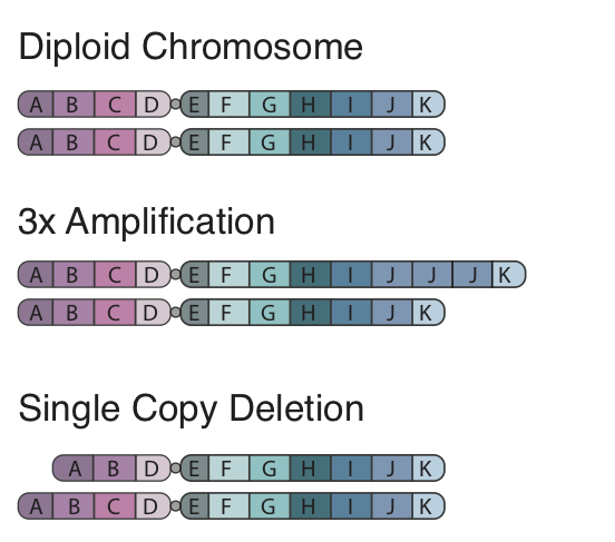
To begin, the concept of a CNA is fairly straight forward, in the figure to the left we show a standard pair of chromosomes divided into 8 segments. In a copy number amplification a region of the genome is duplicated, in our figure region J has 2 extra segments right after each other. When looking at this region in the reference genome we would expect to see a sharp and dramatic increase in coverage at this region. Further with paired end data the insert size for reads spanning the amplification would be larger. In contrast a deletion is how it sounds and is simply a segment of the chromosome which is gone. In our figure we show a single copy deletion of segment C which would result in a sharp drop in coverage at that region in the sequencing data and a shorter average insert size at the breakpoints of the event.

Somatic CNA for WGS

copyCat is an R package used for detecting somatic (experiment/control) copy number aberrations. It works by measuring the depth of coverage from a sequencing experiment. For example in a diploid organism such as human, a single copy number deletion should result in aproximately half the depth (number of reads) compared to the control. Before we run copyCat we need to obtain depth calculations corresponding to a specific window size for our sequencing data. We can use mosdepth for this task. The paramters we give to mosdepth are described below, to run with copyCat we also need to decompress the output from mosdepth and manipulate the output such that it has three columns with header names “Chr”, “Start”, “Counts.$average_read_size” (i.e. Counts.100).

mosdepth paramters:

–no-per-base: omit the per base depth calculation and only calculate depth per region (makes mosdepth run much faster)
-t: number of threads to use
-b: window size for calculating depth
output directory
bam file

# make directory to store copycat results
mkdir -p ~/workspace/somatic/copycat_wgs
cd ~/workspace/somatic/copycat_wgs

# run mosdepth for tumor/normal
mosdepth --no-per-base -t 4 -b 10000 ~/workspace/somatic/copycat_wgs/WGS_Norm.mosdepth ~/workspace/align/WGS_Norm_merged_sorted_mrkdup_bqsr.bam
bgzip -d WGS_Norm.mosdepth.regions.bed.gz
cat ~/workspace/somatic/copycat_wgs/WGS_Norm.mosdepth.regions.bed | cut -f 1,2,4 | awk 'BEGIN{print "Chr\tStart\tCounts.100"}1' > ~/workspace/somatic/copycat_wgs/WGS_Norm.mosdepth.regions.2.bed

mosdepth --no-per-base -t 4 -b 10000 ~/workspace/somatic/copycat_wgs/WGS_Tumor.mosdepth ~/workspace/align/WGS_Tumor_merged_sorted_mrkdup_bqsr.bam
bgzip -d WGS_Tumor.mosdepth.regions.bed.gz
cat ~/workspace/somatic/copycat_wgs/WGS_Tumor.mosdepth.regions.bed | cut -f 1,2,4 | awk 'BEGIN{print "Chr\tStart\tCounts.100"}1' > ~/workspace/somatic/copycat_wgs/WGS_Tumor.mosdepth.regions.2.bed

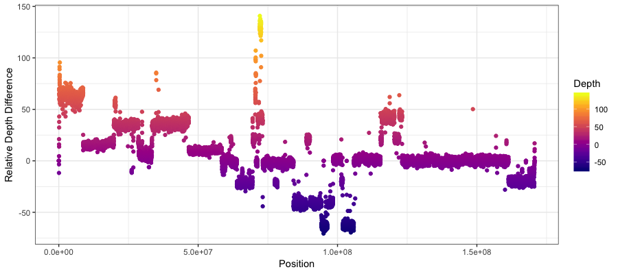
Having run mosdepth we have the core data we need to determine copy number. Let’s go ahead and quickly examine a chromosome to get an idea of what we’re looking at. The below code will make a crude adjustment to normalize the data based on the number of reads present in the samples and plot the result for chromosome 6.

# start R
R

# set working directory
setwd("~/workspace/somatic/copycat_wgs")

# load libraries
library(ggplot2)
library(data.table)
library(viridis)

# read in the depth depth data
tumor_depth <- fread("WGS_Tumor.mosdepth.regions.2.bed")
normal_depth <- fread("WGS_Norm.mosdepth.regions.2.bed")

# merge the two
all_depth <- merge(tumor_depth, normal_depth, by=c("Chr", "Start"), suffixes=c("Tumor", "Normal"))

# normalize the data based on number of reads
total_tumor_reads <- sum(all_depth$Counts.100Tumor)
total_normal_reads <- sum(all_depth$Counts.100Normal)
all_depth$Counts.100Normal <- all_depth$Counts.100Normal * (total_tumor_reads/total_normal_reads)

# calculate the difference in depth between tumor and normal
all_depth$diff <- all_depth$Counts.100Tumor - all_depth$Counts.100Normal

# plot the result for chromosome 6
pdf(file="tumor_depth_cn.chr6.pdf", height=5, width=10)
ggplot(all_depth[all_depth$Chr == "chr6",], aes(x=Start, y=diff, color=diff)) + geom_point() + scale_color_viridis("Depth", option = "plasma") + theme_bw() +
    ylab("Relative Depth Difference") + xlab("Position")
dev.off()

# quit R
q() # don't save workspace image: n [ENTER]

you should see something like the plot below where there is a fairly clear indication of a copy number amplification on the p arm of the chromosome, and a copy deletion twoards the center of the chromosome. Keep in mind that what’s plotted is the Tumor depth relative to the normal and not the actual copy number.

Nice job, that was pretty easy! But not so fast, there are two obvious biases when using depth to determine copy number. The first, GC-content is well known to have an effect on coverage in illumina sequencing data. This goes all the way back to the PCR amplification of the library affecting the number of reads generated. The second thing which can introduce bias is the overall mapability of a region of the genome. A low complexity region in the genome for example will have coverage differences just because it is hard for alignment algorithms to map reads there. These biases are fairly straight forward to address in WGS data however in exome/targeted data it is much more complicated.

The copyCat package is able to adjust for these biases in WGS data and is what we’ll start with. To start with copyCat we need to obtain GC content and mapability scores for our data. Fortunately the author of copyCat has a script to create these annotation files. As our first step let’s go ahead and download the script into the workspace/bin directory and extract the contents.

cd /workspace/bin
wget -c http://genomedata.org/pmbio-workshop/misc/createCustomAnnotations.zip
unzip createCustomAnnotations.zip

Now that we’ve got everything set up we can run the script runEachChr.sh to create these mapability and gc content annotations, but first lets talk about what the script is actually doing. To create the mapability annotations it first takes the a single record fasta (i.e. for a single chromosome) and generates all possible combination of reads for a given read length (in our case the read length is 100 bp). It then takes these reads and aligns them to the multi record fasta (i.e. the whole genome) to determine which of these reads map uniquely to where they belong. If a read were to be mapped anywhere else from where it originally came from in the single record fasta that would be indicitive of a lower mapability at the region where that read was originally derived. The gc content annotation is the proportion of bases which are either a guanine or cytosine for a given region. The instructions for running this script can be found in the README however to sumarize the script will take the following positional arguments:

single record fasta (i.e. chr6)
multi record fasta (i.e. full genome)
average length of reads (for us this is 100)
entrypoint file (chromosome boundaries)
output directory

The script will create a directory called copyCat_annotation with annotations formatted and structured in the appropriate way. This script takes a couple hours to run so we provide the results which you can download from genomedata.org. We also will need to add a gaps.bed file specifying the coordinates for regions to ignore (i.e. telomeres, etc.). A version of this is also made available by the author of copyCat and so we will download this file as well and modify it slightly such that our chromosome names begin with chr. This file should be place at the top level of the copycat annotation directory.

## run the script to create the annotation dir
# cd /workspace/setup/bin/createCustomAnnotations.v1
# grep "chr6\|chr17" hg38entrypoints.female > hg38entrypoints.2.female
# bash runEachChr.sh /workspace/inputs/references/genome/ref_genome_split/chr6.fa /workspace/inputs/references/genome/ref_genome.fa 100 hg38entrypoints.female /workspace/somatic/copycat_wgs
# bash runEachChr.sh /workspace/inputs/references/genome/ref_genome_split/chr17.fa /workspace/inputs/references/genome/ref_genome.fa 100 hg38entrypoints.female /workspace/somatic/copycat_wgs

## download the gaps.bed file
# cd /workspace/somatic/copycat_wgs/copyCat_annotation
# wget -c https://xfer.genome.wustl.edu/gxfer1/project/cancer-genomics/copyCat/GRCh38/gaps.bed
# cat gaps.bed | awk '{print "chr"$0}' > tmp && mv tmp gaps.bed

## rename the entrypoints file
# mv hg38entrypoints.female entrypoints.female
# cp entrypoints.female entrypoints.male

# as mentioned the above takes some time so we'll just download the result for HG38
cd /workspace/somatic/copycat_wgs
wget -c http://genomedata.org/pmbio-workshop/misc/copyCat_annotation.zip
unzip copyCat_annotation.zip

At the end your directory structure should look something like this:

cd /workspace/somatic/copycat_wgs/copyCat_annotation && tree
.
├── entrypoints.female
├── entrypoints.male
├── gaps.bed
└── readlength.100
    ├── gcWinds
    │   ├── chr17.gc.gz
    │   └── chr6.gc.gz
    └── mapability
        ├── chr17.dat.gz
        └── chr6.dat.gz

With Everything now set up we can start R and load the copyCat library. From there we can run the runPairedSampleAnalysis() function to perform the analysis. Most of the parameters in the function are the defaults and are only provided for the sake of completeness, the parameters changed are as follows:

annotationDirectory: the path to the mapability and gc annotations we created from the bash script
outputDir: whre to write our output
normal: path to the normal mosdepth based depth calculations
tumor: path to the tumor mosdepth based depth calculations
maxCores: number of cores to use, 0 means all available cores

# change dir and Start R
cd /workspace/somatic/copycat_wgs/
R

# load the copyCat library
library(copyCat)

# run copyCat in paired mode
runPairedSampleAnalysis(annotationDirectory="/workspace/somatic/copycat_wgs/copyCat_annotation",
                        outputDirectory="/workspace/somatic/copycat_wgs",
                        normal="/workspace/somatic/copycat_wgs/WGS_Norm.mosdepth.regions.2.bed",
                        tumor="/workspace/somatic/copycat_wgs/WGS_Tumor.mosdepth.regions.2.bed",
                        inputType="bins",
                        maxCores=0,
                        binSize=0,
                        perLibrary=1,
                        perReadLength=1,
                        verbose=TRUE,
                        minWidth=3,
                        minMapability=0.6,
                        dumpBins=TRUE,
                        doGcCorrection=TRUE,
                        samtoolsFileFormat="unknown",
                        purity=1,
                        normalSamtoolsFile=NULL,
                        tumorSamtoolsFile=NULL)
# exit R
q()

The analysis will take a few minutes to complete however once it’s done there are a few files that we care about. First you’ll notice there is now a plots directory at /workspace/somatic/copycat_wgs/plots, inside we can view the graphs copyCat created to visualize the gc bias correction, they should look something like this:

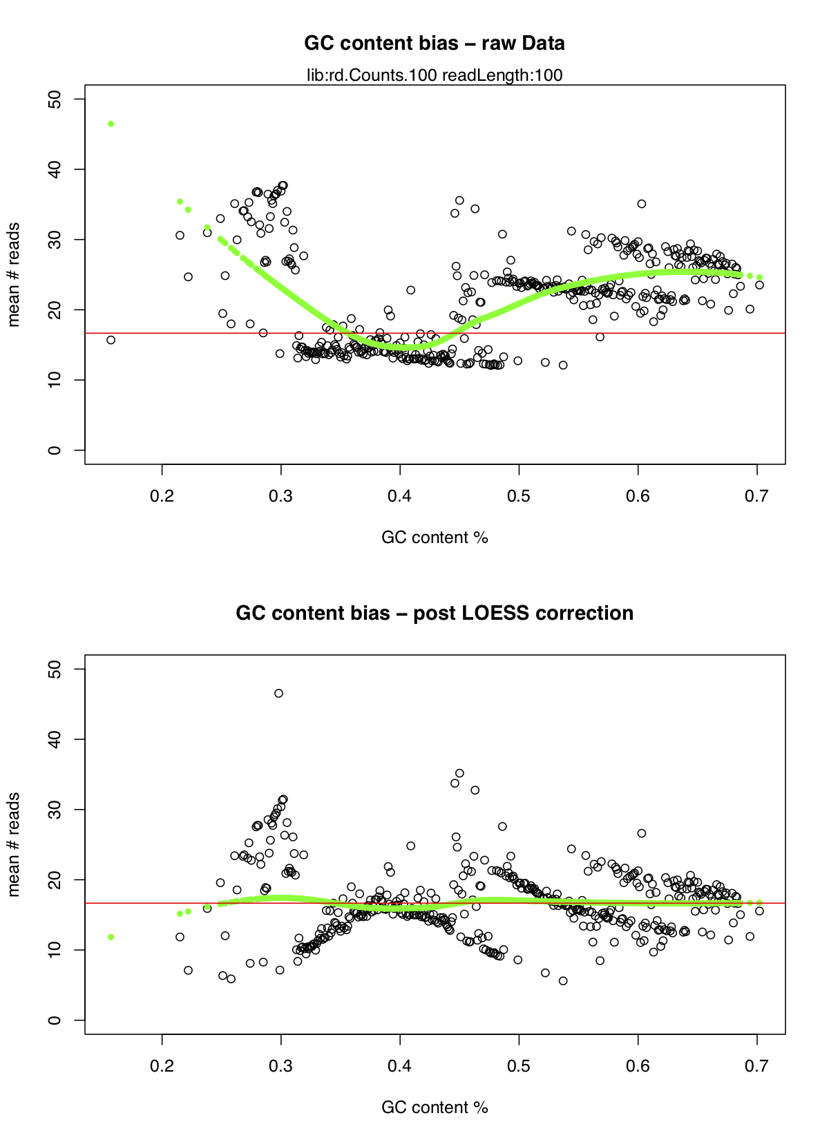
As we can see there was quite an extreme bias between the number of reads mapped and the GC content of the reads particulary when the GC content falls below 30% or above 50% however the LOESS correction dealt with this quite nicely.

Next let’s look at the actual copy number calls from copyCat. There are three files output files that we care about here:

rd.bins.dat: contains the chromsome, position and the inferred tumor CN where 2 represents a normal diploid state
segs.paired.dat: contains the result of the segmentation algorithm with columns “chromosome”, “start”, “stop”, “windows”, “inferred tumor CN”
alts.paired.dat: is identical to segs.paired.dat however those segments which are copy neutral are removed.

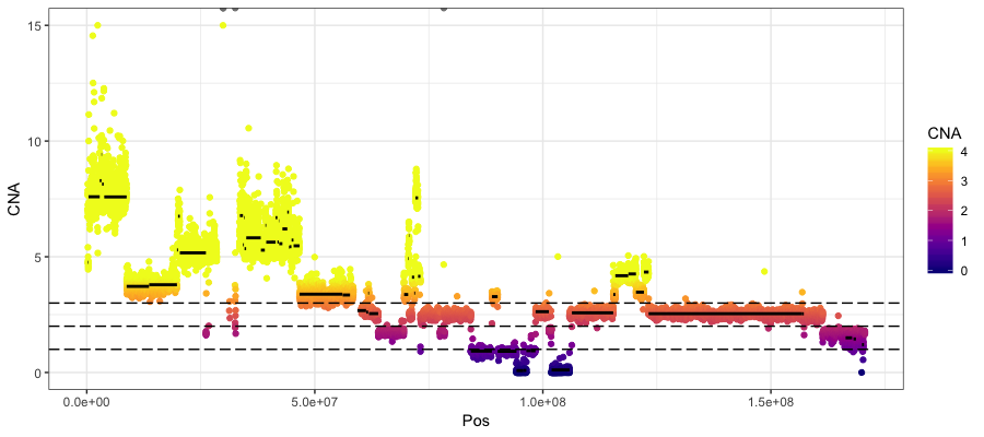
As a final step lets load R and plot the results for chromosome 6.

# start R
R

# set working directory
setwd("/workspace/somatic/copycat_wgs")

# load libraries
library(ggplot2)
library(data.table)
library(viridis)
library(scales)

# read in the data
copy_segment_alteration <- fread("alts.paired.dat")
colnames(copy_segment_alteration) <- c("Chr", "Start", "Stop", "Windows", "Tumor_CN")
cna_bin <- fread("rd.bins.dat")
colnames(cna_bin) <- c("Chr", "Pos", "CNA")

# create the plot
pdf(file="copycat_final.chr6.pdf", height=5, width=10)
ggplot() + geom_point(data=cna_bin[cna_bin$Chr == "chr6",], aes(x=Pos, y=CNA, color=CNA)) +
    geom_segment(data=copy_segment_alteration[copy_segment_alteration$Chr == "chr6",], aes(x=Start, xend=Stop, y=Tumor_CN, yend=Tumor_CN), color="black", size=1) +
    scale_y_continuous(limits=c(0, 15), oob=squish) + scale_color_viridis(limits=c(0, 4), option="plasma", oob=squish) + theme_bw() +
    geom_hline(yintercept = c(1, 2, 3), linetype="longdash")
dev.off()
# exit R
q()

Somatic CNA for exome

CNVkit is a python package for copy number calling specifically designed for hybrid capture and exome sequencing data. During a typical hybrid capture sequencing experiment the probes capture DNA from the sequencing library, however the probes don’t always bind perfectly. This results in not only the “on-target” regions being pulled from the library for later sequencing but “off-target” as well where the probes didn’t perfectly bind and essentially pulled the wrong region. The effect provides very low read coverage across the entire genome which CNVkit takes advantage of to make CN calls. Further the software performs the basic bias correction for gc-content and mappability discussed above and will also correct for the typically normal distrubtion of reads for a given target region and the spacing between them.

To start lets for make a directory to store our results and then activate the conda environemnt which has CNVkit.

# make directory to store results
mkdir -p ~/workspace/somatic/cnvkit_exome
cd ~/workspace/somatic/cnvkit_exome

# activate the cnvkit conda environment
source activate cnvkit

Our next step is to calculate the regions of the genome which are inaccessible to sequencing, typically this includes telomeres, centromeres and other highly repetitive regions. We will use the command cnvkit.py access for this and give it specific regions to exclude as well which we know are problematic. The arguments cnvkit.py takes for this are as follows:

Path to fasta file containing the reference
-x: Path to bed file containing specific regions to exclude
-o: output file

# Calculate the regions of the genome which are inaccessible to sequencing
cnvkit.py access ~/workspace/inputs/references/genome/ref_genome.fa -x ~/workspace/somatic/copycat_wgs/copyCat_annotation/gaps.bed -o ~/workspace/inputs/references/genome/access-excludes.hg38.bed

# cnvkit will complain if access-excludes contains chromosomes not in the bam file
# we subset to chr6 and chr17 here to avoid this error later
grep "chr6\|chr17" ~/workspace/inputs/references/genome/access-excludes.hg38.bed > ~/workspace/inputs/references/genome/access-excludes.hg38.chr6_and_17.bed

With our accessibility file created we can run cnvkit.py batch which will run the entire cnvkit pipeline for us, though we could of course run each command in the pipeline separetly if we wanted more control. The parameters to run this pipeline are as follows:

Path to tumor bam file
–normal: Path to normal bam file (to run in paired mode)
–targets: Target file corresponding to the exome probes, we created this in module 2
–fasta: fasta file corresponding to the reference
–access: the accessibility file created above
–output-reference: where to store the output reference file the pipeline creates/uses
–output-dir: where to store the results from the pipeline
–method hybrid: specifies what mode to run in, hybrid capture for our exome reagent
-p 20: Number of threads to use
–diagram: specifies to create a diagram of the results
–scatter: specifies to create a scatter plot of the results
–drop-low-coverage: specifies to drop low coverage bins (don’t use in germline mode!)

We will also convert the pdf diagram and scatter plots to png so that they load faster.

# cnvkit will complain if chromosomes are in the bed file but not the bam, we fix this here
grep "chr6\|chr17" ~/workspace/inputs/references/exome/SeqCap_EZ_Exome_v3_hg38_primary_targets.v2.sort.merge.bed > ~/workspace/inputs/references/exome/SeqCap_EZ_Exome_v3_hg38_primary_targets.v2.chr6_and_17.bed

# run the entire cnvkit workflow for the exome data
cnvkit.py batch ~/workspace/align/Exome_Tumor_sorted_mrkdup_bqsr.bam --normal ~/workspace/align/Exome_Norm_sorted_mrkdup_bqsr.bam --targets ~/workspace/inputs/references/exome/SeqCap_EZ_Exome_v3_hg38_primary_targets.v2.chr6_and_17.bed --fasta ~/workspace/inputs/references/genome/ref_genome.fa --access ~/workspace/inputs/references/genome/access-excludes.hg38.chr6_and_17.bed --output-reference ~/workspace/inputs/references/genome/my_reference.cnn --output-dir ~/workspace/somatic/cnvkit_exome/ --method hybrid -p 8 --diagram --scatter --drop-low-coverage

# convert the pdf generated from the workflow to png/jpg
convert Exome_Tumor_sorted_mrkdup_bqsr-scatter.pdf Exome_Tumor_sorted_mrkdup_bqsr-scatter.png
convert Exome_Tumor_sorted_mrkdup_bqsr-scatter.pdf Exome_Tumor_sorted_mrkdup_bqsr-scatter.jpg

convert Exome_Tumor_sorted_mrkdup_bqsr-diagram.pdf Exome_Tumor_sorted_mrkdup_bqsr-diagram.png
convert Exome_Tumor_sorted_mrkdup_bqsr-diagram.pdf Exome_Tumor_sorted_mrkdup_bqsr-diagram.jpg

With our running of the pipeline completed you should see the files listed below in your output directory. For a complete description of the files and the specific columns please see the CNVkit file format help documentation available here.

Exome_Norm_sorted_mrkdup.antitargetcoverage.cnn -> antitarget bin coverage for normal
Exome_Norm_sorted_mrkdup.targetcoverage.cnn -> target bin coverage for normal
Exome_Tumor_sorted_mrkdup-diagram.pdf -> diagram of CN calls
Exome_Tumor_sorted_mrkdup-scatter.pdf -> scatter plot of CN calls
Exome_Tumor_sorted_mrkdup.antitargetcoverage.cnn -> antitarget bin coverage for tumor
Exome_Tumor_sorted_mrkdup.cnr -> Bin-level log2 ratios
Exome_Tumor_sorted_mrkdup.cns -> Segmented log2 ratios
Exome_Tumor_sorted_mrkdup.targetcoverage.cnn -> target bin coverage for tumor

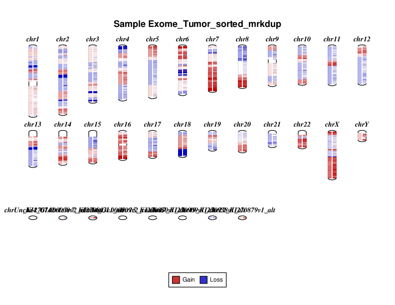
Let’s take a look at the plots that were produced. Below you will see the cnvkit diagram results for the entire exome region. Your results will look a bit different as you only ran a subset of the data. On the left of each chromosome in the diagram amplifications (red) and deletions (blue) are displayed on the left side of each chromosome. On the right side the individual bins for each CN call are displayed.

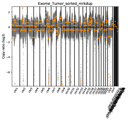
The scatter plot shows the same general information as the diagram but in a slightly different fashion. On the y-axis we have the log2 ratio of T/N CN calls. Let’s go over this a bit as it can get a bit confusing. In our case we have a typical diploid genome (i.e. each chromosome has 2 copies), so in a signle sample copy-neutral would be 2. The y-axis is displaying the log2 ratio of T/N so copy neutral would be log2(2/2) which is 0. Each grey dot is a binned CN call and orange lines are segments. The x-axis is obviously the coordinate for the CN bin.

Finally it might be the case that you want a closer look at the results, perhaps theres a specific region of interest that you would like to view in detail. Let’s go ahead and make both a chromosome 6 scatter plot and heatmaps for both the probes and segment calls. We can use cnvkit.py scatter and cnvit.py heatmap to achieve this.

# create a scatter plot for just chromosome 6
cnvkit.py scatter --segment Exome_Tumor_sorted_mrkdup_bqsr.cns --chromosome chr6:1-170805979 --output chr6_scatter.pdf Exome_Tumor_sorted_mrkdup_bqsr.cnr

# create a heatmap for just chromosome 6
cnvkit.py heatmap --chromosome chr6:1-170805979 --output chr6_heatmap_probes.pdf Exome_Tumor_sorted_mrkdup_bqsr.cnr
cnvkit.py heatmap --chromosome chr6:1-170805979 --output chr6_heatmap_segments.pdf Exome_Tumor_sorted_mrkdup_bqsr.cns

# deactivate conda environment
source deactivate

It should be noted that cnvkit.py can also work on whole genome sequencing data. To run we can do the same exact cnvkit.py batch command as above with the modification that we will need to change the --method to wgs and obviously change the input data to be WGS.

# make directory to store results
mkdir -p /workspace/somatic/cnvkit_wgs
cd /workspace/somatic/cnvkit_wgs

# activate cnvkit environment
source activate cnvkit

# run the cnvkit pipeline
cnvkit.py batch ~/workspace/align/WGS_Tumor_merged_sorted_mrkdup_bqsr.bam --normal ~/workspace/align/WGS_Norm_merged_sorted_mrkdup_bqsr.bam --fasta ~/workspace/inputs/references/genome/ref_genome.fa --access ~/workspace/inputs/references/genome/access-excludes.hg38.chr6_and_17.bed --output-reference ~/workspace/inputs/references/genome/my_reference.cnn --output-dir /workspace/somatic/cnvkit_wgs/ --method wgs -p 8 --diagram --scatter

# deactivate the cnvkit environment
source deactivate

# convert the .pdf plots to png/jpg
convert WGS_Tumor_merged_sorted_mrkdup_bqsr-scatter.pdf WGS_Tumor_merged_sorted_mrkdup_bqsr-scatter.png
convert WGS_Tumor_merged_sorted_mrkdup_bqsr-scatter.pdf WGS_Tumor_merged_sorted_mrkdup_bqsr-scatter.jpg

convert WGS_Tumor_merged_sorted_mrkdup_bqsr-diagram.pdf WGS_Tumor_merged_sorted_mrkdup_bqsr-diagram.png
convert WGS_Tumor_merged_sorted_mrkdup_bqsr-diagram.pdf WGS_Tumor_merged_sorted_mrkdup_bqsr-diagram.jpg

« Somatic SV Filtering/Annotation/Review Course Somatic CNV Filtering/Annotation/Review »