Somatic LOH Filtering/Annotation/Review
Module objectives
- Find segments of chromosomes 17 that show LOH
Get list of breast cancer genes on chromosome 17
Before we get our segmentation results, we will use a list of known breast cancer genes from the Cancer Gene Census to extract info for plotting these genes against our segmentation results.
# Download tsv file with known breast cancer genes on chromosome 17
wget http://genomedata.org/pmbio-workshop/references/CGC/chr17_breast_cancer_genes.tsv

# Create list of gene names
awk '{print $1}' chr17_breast_cancer_genes.tsv > chr17_breast_cancer_gene_names

# Filter gtf file down to chromosome 17 genes
awk '$1 == "chr17" && $3 == "gene"' /workspace/inputs/references/transcriptome/ref_transcriptome.gtf > chr17_ref_transcriptome.gtf

# Remove " " from gene names in gtf file
sed 's/[";]/ /g' chr17_ref_transcriptome.gtf > tmp.file
mv tmp.file chr17_ref_transcriptome.gtf

# Search gtf file for breast cancer genes
awk 'BEGIN {while ((getline <"chr17_ref_transcriptome.gtf") > 0) {REC[$14]=$0}} {print REC[$1]}' < chr17_breast_cancer_gene_names > chr17_breast_cancer_genes.gtf

# Subset file down to columns needed for plotting later
awk '{print $1 "\t" $4 "\t" $5 "\t" $14}' chr17_breast_cancer_genes.gtf > chr17_breast_cancer_genes.table
Run DNAcopy
To find regions of LOH, we will use an R package for analyzing copy number variations, DNAcopy.
# Start R
R

# Set working directory
setwd("/workspace/somatic/loh")

# Load libraries
library(dplyr); library(tidyr); library(ggplot2); library(DNAcopy)

# Read table with tumor VAFs into R
tumor <- read.delim("tumor.VAFs.table", header = TRUE, col.names = c("CHROM", "POS", "TUMOR_DP", "AD", "VAF"))

# Make sure tumor VAFs are numeric for calculations
tumor$VAF <- as.numeric(tumor$VAF)

# Create column for abs(.5 - tumor VAF)
tumor$ABS <- abs(.5 - tumor$VAF)

# Create CNA.object for DNAcopy segmentation analysis, Note: this step will give a warning about repeated maploc, we can ignore this warning
LOH_CNA.object <- CNA(genomdat = tumor$ABS, chrom = tumor$CHROM, maploc = tumor$POS, data.type = 'binary')

# Run segmentation analysis
LOH.segmentation <- segment(LOH_CNA.object)
LOH.segmentation.output <- LOH.segmentation$output

# Extract columns needed to plot segmentation results, change column names
LOH_segments <- select(LOH.segmentation.output, chrom, loc.start, loc.end, seg.mean)
colnames(LOH_segments) <- c("CHROM", "START", "END", "MEAN")

# Create columns for .5 + segment means, .5 - segment means
LOH_segments$TOP <- .5 + LOH_segments$MEAN; LOH_segments$BOTTOM <- .5 - LOH_segments$MEAN

# Read in table with germline VAFs for plotting
germline <- read.delim("heterozygous.snps.table", header = TRUE, col.names = c("CHROM", "POS", "GT", "AD", "DP", "VAF"))

# Read in table with cancer gene info for plotting
cancer_genes <- read.delim("chr17_breast_cancer_genes.table", header = FALSE, col.names = c("CHROM", "START", "END", "GENE"))

# Plot VAFs, LOH segments, breast cancer genes for chromosome 17
pdf("chr17_segmentation.pdf", width = 11.5, height = 2.75)
chr17_segment_plot <- ggplot() + geom_point(data = germline, aes(POS,VAF), color="blue", size = .75) + geom_point(data = tumor, aes(POS,VAF), color="green", size = .75) + geom_segment(data = LOH_segments, aes(x = LOH_segments$START,y = LOH_segments$TOP,xend = LOH_segments$END,yend = LOH_segments$TOP), size = 1) + geom_segment(data = LOH_segments, aes(x = LOH_segments$START,y = LOH_segments$BOTTOM,xend = LOH_segments$END,yend = LOH_segments$BOTTOM), size = 1) + geom_segment(data = cancer_genes, aes(x = cancer_genes$START, y = 1.2, xend = cancer_genes$END, yend = 1.2), size = 3, color = "red", na.rm = TRUE) + geom_text(data = cancer_genes, aes(x=END, y=1.35, label=GENE), size = 2, color = "red", angle = 45, na.rm = TRUE) + xlab("Chromosome Position") + ylab("VAF") + ylim(0, 1.4)
plot(chr17_segment_plot)
dev.off()

# Exit R, no need to save workspace
q()
In your loh directory, you should now see a new file: chr17_segmentation.pdf
The plot you created should look similar to this plot:
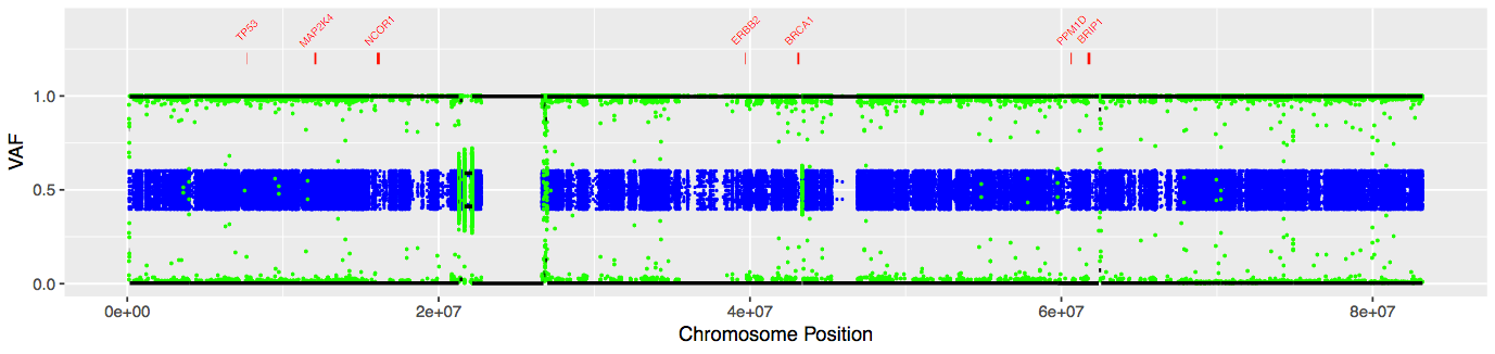
Blue is our normal heterozygous VAFs, green is our tumor VAFs, red is known breast cancer genes, and black is our segmentation results. Black lines close to 0 or 1 indicate segments of complete LOH, while lines between .4 to .6 indicate regions that are still heterozygous. As we can see, chromosome 17 exhibits nearly complete LOH in our tumor sample.
If we had done our LOH analysis on chromosome 6, we would have seen a plot similar to this:
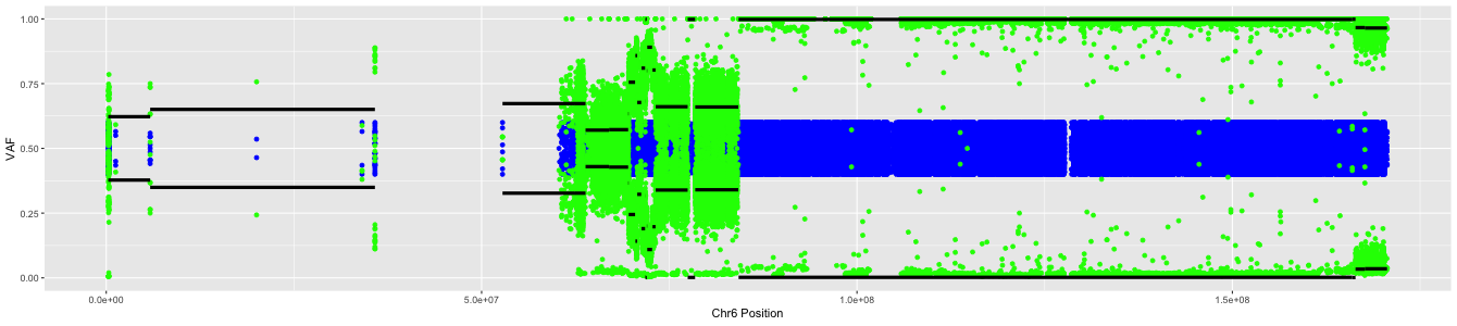
Here, we see regions that are still heterozygous as well as regions of LOH.