Somatic LOH Calling
Module objectives
- Calculate VAFs in normal sample, find heterozygyous germline positions
- Run bam-readcount on tumor sample, use readcounts to calculate tumor VAFs at heterozygous positions
- Determine segments of LOH in tumor sample
Run GATK SelectVariants
First, we will extract all SNPs from the VQSR-filtered whole genome VCF file created in the Germline section.
# Make sure you are in directory for somatic results
cd /workspace/somatic

# Create directory for LOH results, move into that directory
mkdir loh
cd loh

# Extract SNPs
gatk --java-options '-Xmx64g' SelectVariants -R /workspace/inputs/references/genome/ref_genome.fa -V /workspace/germline/WGS_Norm_HC_calls_recalibrated.PASS.vcf -select-type SNP -O WGS_Norm_HC_calls.recalibrated.PASS.snps.vcf
Run GATK VariantsToTable
Next, we will extract the columns with the data we will need for calculating VAFs and determining positions of heterozygosity.
# Create table with columns for chromosome, position, genotype, allele depth, total depth
gatk --java-options '-Xmx64g' VariantsToTable -V WGS_Norm_HC_calls.recalibrated.PASS.snps.vcf -F CHROM -F POS -GF GT -GF AD -GF DP -O WGS_Norm_HC_calls.recalibrated.PASS.snps.table
Calculate VAFs and find heterozygous positions
Now, we will use R to calulate the variant allele frequencies for each allele at each position, then we will get a list of heterozygous positions by filtering our data to positions with VAFs from 40% to 60% allele frequency.
# Start R
R

# Set working directory
setwd("/workspace/somatic/loh")

# Load libraries, Note: ";" separates commands so we can run multiple commands in one line
library(dplyr); library(tidyr)

# Read in table made with VariantsToTable command
normal_calls <- read.delim("WGS_Norm_HC_calls.recalibrated.PASS.snps.table", header = TRUE, col.names = c("CHROM", "POS", "GT", "GT_AD", "DP"))

# Filter for positions with at least 20x coverage
normal_calls <- subset.data.frame(normal_calls, DP >= 20)

# Split GT_AD column, make three new columns with one allele depth per column
normal_calls <- normal_calls %>% separate(GT_AD, c("AD_1", "AD_2", "AD_3"), remove = FALSE, fill = "right")

# Make sure allele depth columns are numeric so they can be used to calculate VAFs
normal_calls$AD_1 <- as.numeric(normal_calls$AD_1); normal_calls$AD_2 <- as.numeric(normal_calls$AD_2); normal_calls$AD_3 <- as.numeric(normal_calls$AD_3)

# Calculate VAFs, allele depth/total dpeth
normal_calls$VAF_1 <- normal_calls$AD_1/normal_calls$DP; normal_calls$VAF_2 <- normal_calls$AD_2/normal_calls$DP; normal_calls$VAF_3 <- normal_calls$AD_3/normal_calls$DP

# Split into separate files for each VAF, remerge so we have one column with all VAFs to filter for heterozygous variants
VAF_1 <- select(normal_calls, CHROM, POS, GT, AD_1, DP, VAF_1); VAF_2 <- select(normal_calls, CHROM, POS, GT, AD_2, DP, VAF_2); VAF_3 <- select(normal_calls, CHROM, POS, GT, AD_3, DP, VAF_3)
colnames(VAF_1) <- c("CHROM", "POS", "GT", "AD", "DP", "VAF"); colnames(VAF_2) <- c("CHROM", "POS", "GT", "AD", "DP", "VAF"); colnames(VAF_3) <- c("CHROM", "POS", "GT", "AD", "DP", "VAF")
normal_calls <- merge(VAF_1, VAF_2, all = TRUE); normal_calls <- merge(normal_calls, VAF_3, all = TRUE)

# Filter for heterozygous posistions, i.e. positions with VAF between .4 and .6
normal_calls <- subset.data.frame(normal_calls, VAF >= .4); normal_calls <- subset.data.frame(normal_calls, VAF <= .6)

# Create table containing info for heterozygous SNPs, will use later to plot results
write.table(normal_calls, file="heterozygous.snps.table", sep = "\t", col.names = TRUE, row.names = FALSE, quote = FALSE)

# Get list of heterozygous positions to use with bam-readcount
heterozygous.positions <- unique(normal_calls[c("CHROM", "POS")])
write.table(heterozygous.positions[ ,c("CHROM", "POS", "POS")], file = "heterozygous.positions.txt", sep="\t", col.names = FALSE, row.names = FALSE, quote = FALSE)

# Exit R, you do not need to save workspace
q()
You should now see two new files in your loh directory:
- heterozygous.snps.table - we will use this for plotting later
- heterozygous.positions.txt - we will use this with bam-readcount
Run bam-readcount
Next, to get the data needed to calculate VAFs in our tumor sample, we will run bam-readcount. The inputs needed for bam-readcount are our reference fasta file, our whole genome bam file, and our position list.
# Run bam-readcount
bam-readcount -w 1 -b 20 -q 20 -f /workspace/inputs/references/genome/ref_genome.fa -l heterozygous.positions.txt /workspace/align/WGS_Tumor_merged_sorted_mrkdup_bqsr.bam chr17 > tumor.readcounts
Calculate tumor VAFs
Now we will use output from bam-readcount to calculate tumor VAFs in R.
# Start R
R

# Set working directory
setwd("/workspace/somatic/loh")

# Load libraries
library(dplyr); library(tidyr); library(ggplot2)

# Read bam-readcount output into R
tumor_VAFs <- read.delim("tumor.readcounts", header = FALSE, fill = TRUE, col.names = c("CHROM", "POS", "REF", "TUMOR_DP", "5", "count_A", "count_C", "count_G", "count_T", "11", "12", "13", "14"))

# Select columns relevant to our calculation
tumor_VAFs <- select(tumor_VAFs, CHROM, POS, TUMOR_DP, count_A, count_C, count_G, count_T)

# Filter down to positions with at least 20x coverage
tumor_VAFs <- subset.data.frame(tumor_VAFs, TUMOR_DP >= 20)

# Spilt columns with allele info into separate columns with allele depth
tumor_VAFs <- tumor_VAFs %>% separate(count_A, c("A", "A_AD"), extra = "drop"); tumor_VAFs <- tumor_VAFs %>% separate(count_C, c("C", "C_AD"), extra = "drop"); tumor_VAFs <- tumor_VAFs %>% separate(count_G, c("G", "G_AD"), extra = "drop"); tumor_VAFs <- tumor_VAFs %>% separate(count_T, c("T", "T_AD"), extra = "drop")

# Again, select columns relevant to VAF calculation
tumor_VAFs <- select(tumor_VAFs, CHROM, POS, TUMOR_DP, A_AD, C_AD, G_AD, T_AD)

# Make sure allele depth columns are numeric
tumor_VAFs$A_AD <- as.numeric(tumor_VAFs$A_AD); tumor_VAFs$C_AD <- as.numeric(tumor_VAFs$C_AD); tumor_VAFs$G_AD <- as.numeric(tumor_VAFs$G_AD); tumor_VAFs$T_AD <- as.numeric(tumor_VAFs$T_AD)

# Calculate VAFs
tumor_VAFs$VAF_A <- tumor_VAFs$A_AD/tumor_VAFs$TUMOR_DP; tumor_VAFs$VAF_C <- tumor_VAFs$C_AD/tumor_VAFs$TUMOR_DP; tumor_VAFs$VAF_G <- tumor_VAFs$G_AD/tumor_VAFs$TUMOR_DP; tumor_VAFs$VAF_T <- tumor_VAFs$T_AD/tumor_VAFs$TUMOR_DP

# Split into separate files for each VAF, remerge so we have one column with all tumor VAFs
VAF_A <- select(tumor_VAFs, CHROM, POS, TUMOR_DP, A_AD, VAF_A); VAF_C <- select(tumor_VAFs, CHROM, POS, TUMOR_DP, C_AD, VAF_C); VAF_G <- select(tumor_VAFs, CHROM, POS, TUMOR_DP, G_AD, VAF_G); VAF_T <- select(tumor_VAFs, CHROM, POS, TUMOR_DP, T_AD, VAF_T)
colnames(VAF_A) <- c("CHROM", "POS", "TUMOR_DP", "AD", "VAF"); colnames(VAF_C) <- c("CHROM", "POS", "TUMOR_DP", "AD", "VAF"); colnames(VAF_G) <- c("CHROM", "POS", "TUMOR_DP", "AD", "VAF"); colnames(VAF_T)<- c("CHROM", "POS", "TUMOR_DP", "AD", "VAF")
tumor_VAFs <- merge(VAF_A, VAF_C, all = TRUE); tumor_VAFs <- merge(tumor_VAFs, VAF_G, all = TRUE); tumor_VAFs <- merge(tumor_VAFs, VAF_T, all = TRUE)

# Filter out VAFs where no reads mapped (i.e VAFs = 0)
tumor_VAFs <- subset.data.frame(tumor_VAFs, VAF > 0)

# Create table for tumor VAFs
write.table(tumor_VAFs, file="tumor.VAFs.table", sep = "\t", col.names = TRUE, row.names = FALSE, quote = FALSE)

# Read in previously made table with germline VAFs
germline_VAFs <- read.delim("heterozygous.snps.table", header = TRUE, col.names = c("CHROM", "POS", "GT", "AD", "DP", "VAF"))

# Plot VAFs for chromosome 17
pdf("chr17_normal_vs_tumor_VAFs.pdf", width = 11.5, height = 2.75)
chr17_VAF_plot <- ggplot() + geom_point(data = germline_VAFs, aes(POS,VAF), color="blue", size = .75) + geom_point(data = tumor_VAFs, aes(POS,VAF), color="green", size = .75) + xlab("Chromosome Position") + ylab("VAF")
plot(chr17_VAF_plot)
dev.off()

# Exit R, no need to save workspace
q()
You should now see two new files in your loh directory
- tumor.VAFs.table
- chr17_normal_vs_tumor_VAFs.pdf
The plot should look similar to this:
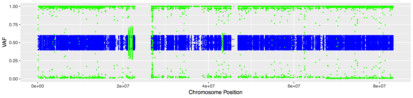
In the next section, we will look for regions of LOH